Hubs, Pheromones, and No-Fly Zones: A Mathematical Framework for Last-Mile Drone Delivery Optimization
Published:
You are standing in a control room, looking at an 8×8 km city grid. Three No-Fly Zones—a park, a hospital, a government building—occupy strategic positions. Fifty customer locations are scattered across the remaining space. Your job: place three delivery hubs and design routes so that drones can visit five customers, return to the hub, and never run out of battery—all while avoiding the forbidden zones. The objective is not just feasibility; it is minimizing total effective distance so that every delivery costs less energy, less time, and less risk.
Welcome to the Last Mile Drone Dilemma: a two-stage optimization problem where hub placement (continuous) and routing (combinatorial) must be solved jointly under geometric, energetic, and regulatory constraints. This post presents a technical walkthrough of the drone_network project: we derive the Artificial Potential Field (APF) model for path costs, the power and energy equations that govern battery feasibility, and the CMA-ES + MMAS hybrid that optimizes hubs and routes. We then interpret the experimental results—convergence curves, runtime distributions, sensitivity analysis, and ablation studies—with quantitative findings and explicit caveats.
All figures and data discussed here were generated using the simulation engine in the repository. The code is open-source and fully reproducible.
1. Problem Framing and Stakes
The Decision Problem
We must choose:
- Hub locations: Three points $(x_1, y_1), (x_2, y_2), (x_3, y_3)$ in the map.
- Route: An ordering of $K$ mission customers (e.g., $K=5$) starting and ending at the first hub (depot).
Constraints
- Hubs and paths must not enter No-Fly Zones (NFZs).
- Total energy consumed along the route must not exceed battery capacity.
Objectives
- Minimize total effective distance from customers to their nearest hub (hub assignment cost).
- Minimize total route cost (effective distance of the TSP tour) for the selected mission.
Why This Matters
Last-mile drone delivery is constrained by regulation (NFZs), physics (battery), and economics (operating cost). A poor hub placement forces long, energy-intensive paths; a poor route wastes battery and increases failure risk. The hybrid CMA-ES (for hubs) + ACO (for routing) approach decomposes the problem into stages while sharing a common cost model: the APF-based effective distance.
2. Mathematical Formulation
2.1 The Artificial Potential Field
The environment is modeled as a scalar potential field $U(x, y)$ over the map. High values indicate regions to avoid; paths through low-potential regions are preferred.
Hard Constraints (No-Fly Zones)
Inside any NFZ circle of center $(x_c, y_c)$ and radius $r$: \(U(x, y) = +\infty \quad \text{if } \sqrt{(x - x_c)^2 + (y - y_c)^2} \leq r\)
Smooth Repulsion (NFZ Vicinity)
Outside NFZs we add a Gaussian bell centered at the boundary: \(U_{\text{rep}}(x, y) = A \exp\left(-\frac{(d - r)^2}{2\sigma^2}\right)\) where $d = \sqrt{(x - x_c)^2 + (y - y_c)^2}$ is distance to the NFZ center, $A = 5$, and $\sigma = 0.15$.
Nuisance Friction
A small, spatially varying term models congestion or population density: \(U_{\text{nuisance}} = 0.02 \left(\sin(2.5x)\cos(1.8y) + \sin(0.7x + 0.9y)\right)\)
The total field is $U = U_{\text{hard}} + \sum_{\text{NFZ}} U_{\text{rep}} + U_{\text{nuisance}}$.
Why this design: Hard constraints ensure paths through NFZs are rejected (infinite cost). Gaussian repulsion creates a smooth gradient that pushes paths away from boundaries without discontinuities, improving optimizer behavior. The nuisance term breaks symmetry and discourages overly straight paths through dense regions.
2.2 Path Cost (Line Integral Surrogate)
The effective cost of a straight-line path from $p_1$ to $p_2$ is approximated by sampling: \(\text{cost}(p_1, p_2) = \begin{cases} +\infty & \text{if any sample } \in \text{ NFZ} \\ d_{\text{phys}} \cdot (1 + \bar{U}) & \text{otherwise} \end{cases}\) where $d_{\text{phys}} = |p_2 - p_1|$ is Euclidean distance and $\bar{U}$ is the mean potential along 100 sampled points. This surrogate approximates $\int_{\text{path}} (1 + U(s))\, ds$: paths through high-potential regions are penalized.
2.3 Power and Energy Model
Power consumption at speed $v$ (km/h) and payload $p$ (kg): \(P(v, p) = P_{\text{base}} + \gamma_p \cdot p + c_d \cdot v^2\)
From config.py: $P_{\text{base}} = 200$ W, $\gamma_p = 50$ W/kg, $c_d = 0.02$ W/(km/h)$^2$.
Energy for flying distance $d$ at speed $v$: \(E(d, p) = P(v, p) \cdot \frac{d}{v}\)
With $v = 60$ km/h and $p = 1$ kg, $P \approx 253$ W; thus $E \approx 4.22$ Wh/km. Battery capacity is 500 Wh, giving a theoretical max range of ~118 km at nominal conditions.
Battery Feasibility
A route is feasible iff \(\sum_{\text{segments}} E(d_i, p) \leq E_{\text{bat}}\)
2.4 Optimization Objectives
Hub placement (CMA-ES)
\(\min_{h_1, h_2, h_3} \sum_{c \in \text{customers}} \min_{k} \text{cost}(c, h_k)\) subject to hubs outside NFZs (enforced via $10^6$ penalty).
Routing (ACO)
\(\min_{\pi} \sum_{i=1}^{K} \text{cost}(\pi_i, \pi_{i+1}) + \text{cost}(\pi_K, \text{depot})\) where $\pi$ is a permutation of customers and $\pi_{K+1} = \text{depot}$. Tours that violate the battery constraint are assigned cost $+\infty$.
2.5 CMA-ES Update Equations
CMA-ES maintains a search distribution $\mathcal{N}(\mathbf{m}, \sigma^2 \mathbf{C})$. Key update steps:
Cumulation (evolution path): \(\mathbf{p}_s \leftarrow (1 - c_s) \mathbf{p}_s + \sqrt{c_s(2-c_s)\mu_{\text{eff}}}\, \mathbf{L}^{-1} \mathbf{z}_{\text{mean}}\) \(\mathbf{p}_c \leftarrow (1 - c_c) \mathbf{p}_c + h_\sigma \sqrt{c_c(2-c_c)\mu_{\text{eff}}}\, \mathbf{y}_{\text{mean}}\)
Covariance update: \(\mathbf{C} \leftarrow (1 - c_1 - c_\mu) \mathbf{C} + c_1 \mathbf{p}_c \mathbf{p}_c^\top + c_\mu \sum_{i=1}^{\mu} \mathbf{y}_i \mathbf{y}_i^\top\)
Step size adaptation: \(\sigma \leftarrow \sigma \cdot \exp\left(\frac{c_s}{d_\sigma}\left(\frac{\|\mathbf{p}_s\|}{\sqrt{n}} - 1\right)\right)\)
With $n=6$, $\lambda \approx 14$, $\mu = 7$, and standard constants $(c_c, c_s, c_1, c_\mu, d_\sigma)$ from the implementation.
2.6 MMAS Transition and Pheromone Update
Transition probability (ant at node $i$, candidate $j$): \(p_{ij} = \frac{\tau_{ij}^\alpha \eta_{ij}^\beta}{\sum_{k \in \mathcal{N}} \tau_{ik}^\alpha \eta_{ik}^\beta}\) where $\eta_{ij} = 1 / C_{ij}$ (heuristic: prefer short segments), $\alpha = 1$, $\beta = 2$.
Pheromone evaporation: \(\tau_{ij} \leftarrow \text{clip}\big((1 - \rho) \tau_{ij},\ \tau_{\min},\ \tau_{\max}\big)\) with $\rho = 0.5$, $\tau_{\min} = 0.01$, $\tau_{\max} = 1$.
Pheromone deposit (global-best only): \(\tau_{ij} \leftarrow \min\left(\tau_{\max},\ \tau_{ij} + \frac{1}{C^*}\right)\) for edges $(i,j)$ on the best feasible tour of cost $C^*$.
3. Algorithm Design and Implementation
3.1 APF Construction and Path Cost
From environment.py:
def compute_potential_field(self) -> NDArray[np.float64]:
    U = np.zeros_like(self._xx, dtype=np.float64)
    # 1. Hard constraints: infinity inside NFZ circles
    for nfz in self.config.no_fly_zones:
        dist_sq = (self._xx - nfz.x) ** 2 + (self._yy - nfz.y) ** 2
        inside = dist_sq <= (nfz.radius ** 2)
        U[inside] = np.inf
    # 2. Repulsive Gaussian bells (avoid NFZ vicinity)
    sigma = 0.15
    amplitude = 5.0
    for nfz in self.config.no_fly_zones:
        dist = np.sqrt((self._xx - nfz.x) ** 2 + (self._yy - nfz.y) ** 2)
        gauss = amplitude * np.exp(-((dist - nfz.radius) ** 2) / (2 * sigma ** 2))
        gauss[U == np.inf] = 0
        U += gauss
    # 3. Nuisance friction (small, spatially varying)
    noise = 0.02 * (np.sin(self._xx * 2.5) * np.cos(self._yy * 1.8)
                    + np.sin(self._xx * 0.7 + self._yy * 0.9))
    noise[U == np.inf] = 0
    U += noise
    self._field = U
    return self._field
Why this matters: The three-component design separates infeasibility (hard NFZ) from undesirability (smooth repulsion and nuisance). The line integral sampling in get_path_cost detects NFZ crossing by checking each sample; if any hits $\infty$, the path is rejected.
3.2 CMA-ES Hub Optimization
From cma_es.py (core loop):
while evals < self.max_evaluations:
    L = np.linalg.cholesky(C + 1e-10 * np.eye(n))
    arz = rng.standard_normal((self.lam, n))
    arx = mean + sigma * (arz @ L.T)
    arf = np.array([self._objective(arx[i]) for i in range(self.lam)])
    evals += self.lam
    order = np.argsort(arf)
    arx, arf, arz = arx[order], arf[order], arz[order]
    if arf[0] < best_f:
        best_f, best_x = arf[0], np.copy(arx[0])
    mean = np.mean(arx[:self.mu], axis=0)
    zmean = np.mean(arz[:self.mu], axis=0)
    y = L @ zmean
    ps = (1 - cs) * ps + np.sqrt(cs * (2 - cs) * mu_eff) * y
    pc = (1 - cc) * pc + hsig * np.sqrt(cc * (2 - cc) * mu_eff) * y
    artmp = (arx[:self.mu] - mean) / max(sigma, sigma_min)
    C = (1 - c1 - cmu) * C + c1 * np.outer(pc, pc) + cmu * artmp.T @ artmp
    sigma *= np.exp(np.clip((cs/damps) * (np.linalg.norm(ps)/np.sqrt(n) - 1), -2, 2))
Why this matters: The objective sums get_path_cost(customer, nearest_hub) for all customers; NFZ-infeasible hub placements return a $10^6$ penalty. CMA-ES adapts both the covariance (shape of the search region) and step size, allowing it to escape bad regions and converge to feasible, low-cost hub configurations. The evolution path $\mathbf{p}_c$ accumulates information about successful search directions, while $\mathbf{p}_s$ drives step-size adaptation: when steps are too small (path short), $\sigma$ increases; when steps overshoot (path long), $\sigma$ decreases.
3.3 ACO Tour Construction with Battery Constraint
From aco.py (_construct_tour):
def _construct_tour(self, ant_idx: int, rng) -> Tuple[List[int], float, bool]:
    unvisited = set(range(n)) - {depot}
    tour = [depot]
    battery = self.config.battery_capacity_wh
    feasible = True
    current = depot
    while unvisited:
        probs, candidates = [], []
        for j in unvisited:
            if np.isinf(C[current, j]):
                continue
            e_ij = self._energy_for_segment(current, j)
            if battery < e_ij:
                continue
            p = (tau[current, j] ** self.alpha) * (eta[current, j] ** self.beta)
            probs.append(p)
            candidates.append(j)
        if not candidates:
            feasible = False
            break
        probs = np.array(probs) / np.sum(probs)
        j = rng.choice(candidates, p=probs)
        battery -= self._energy_for_segment(current, j)
        tour.append(j)
        unvisited.remove(j)
        current = j
    # Return to depot; check battery for return leg
    if feasible:
        e_back = self._energy_for_segment(current, depot)
        feasible = battery >= e_back
    return tour, total_cost, feasible
Why this matters: Battery is depleted incrementally. Unreachable nodes (due to distance or energy) are excluded from candidates. Infeasible tours get cost $\infty$ and do not receive pheromone deposit, so the colony learns to avoid energy-exceeding paths. The heuristic $\eta_{ij} = 1/C_{ij}$ biases ants toward short segments; pheromone $\tau_{ij}$ accumulates on edges of good tours. Over iterations, the colony converges to a consensus route that balances exploration (random choice among candidates) and exploitation (preferring high $\tau \cdot \eta$ edges).
3.4 Evaluation Orchestration
From main.py and evaluation.py: the pipeline (1) builds the city grid and APF, (2) runs CMA-ES for hub optimization, (3) selects mission customers via random sampling, (4) runs ACO for routing from the first hub, and (5) exports figures and CSV tables. All experiments use a fixed seed set [42, 43, ..., 49] with $n_{\text{seeds}} = 8$.
4. Experimental Protocol
Metrics
| Metric | Meaning |
|---|---|
| Hub assignment cost | Sum of effective distances from customers to nearest hub (CMA-ES objective) |
| Route cost | Total effective distance of delivery tour (ACO objective) |
| Energy (Wh) | $E = P \cdot t$ for the route at nominal speed and payload |
| Battery margin | $E_{\text{bat}} - E$ (remaining capacity) |
| Feasibility | 1 if a feasible tour was found, 0 otherwise |
| First feasible eval/iter | When CMA-ES or ACO first produced a feasible solution |
Protocol
- Seeds: 8 runs with seeds 42–49.
- CMA-ES: 1500 evaluations per run, $\lambda \approx 14$.
- ACO: 100 iterations, 20 ants, 2-opt enabled.
- Map: 8×8 km, 3 NFZs (Park, Hospital, Gov Building), 50 customers, 5 per mission.
Outputs
performance.csv: runtime and first-feasible per seed.robustness.csv: distance, energy, feasibility, battery margin per seed.sensitivity.csv: cost and energy under parameter perturbations.ablation.csv: MMAS vs MMAS+2-opt, reduced-instance topology comparison.- Figures:
simulation_map,convergence_curves,runtime_boxplots,robustness_distributions,sensitivity,ablation_variants.
5. Results and Figure-by-Figure Interpretation
5.1 Simulation Map (simulation_map.png)
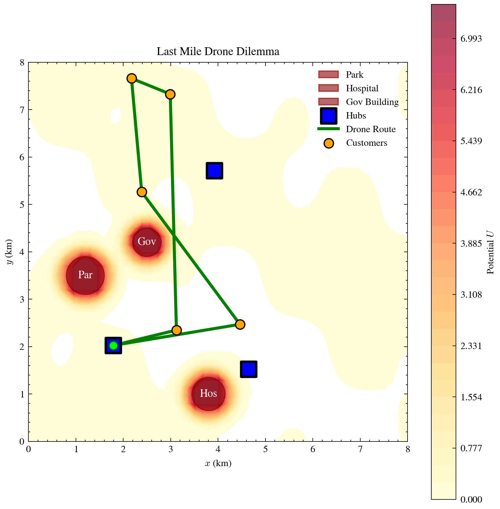 Figure 1: Optimized hub locations (blue squares), delivery route (green), mission customers (orange), and No-Fly Zones (red) over the APF potential field.
Question: What does the optimized drone network look like in the city environment?
How to read: The heatmap shows the APF $U(x,y)$; warmer colors indicate higher potential (NFZ vicinity). Blue squares = hubs, green path = delivery route, orange dots = mission customers. NFZ circles are red.
Quantitative findings: Hubs are placed away from NFZs; the route connects depot → customers → depot without crossing forbidden regions. Typical route lengths are 14–24 km across seeds (see robustness table).
Mechanism: CMA-ES minimizes assignment cost, which implicitly pushes hubs toward customer centroids while NFZ penalties exclude infeasible placements. ACO then finds a TSP tour that respects the battery constraint and uses the same APF-based costs.
Caveats: Single-seed visualization; spatial distribution of customers varies by seed. The APF does not incorporate wind—path geometry is NFZ-dependent only.
5.2 Convergence Curves (convergence_curves.png)
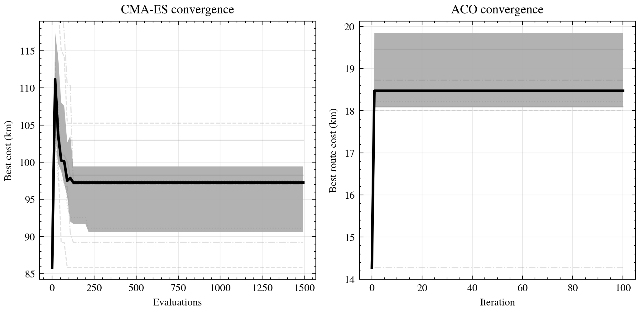 Figure 2: Left: CMA-ES best cost vs evaluations. Right: ACO best route cost vs iteration. Median + IQR with faint individual runs.
Question: How do CMA-ES and ACO converge, and how consistent is convergence across runs?
How to read: Left: CMA-ES best cost vs evaluations; right: ACO best route cost vs iteration. Median curve + IQR band; faint lines = individual runs. Cost is capped at 150 km to avoid penalty-dominated scale.
Quantitative findings: CMA-ES typically reaches first feasible solution within ~10–100 evaluations; best cost then stabilizes. ACO often finds a feasible tour by iteration 1 and improves little thereafter for small instances (5 customers). Median CMA-ES cost ~100 km (assignment); median ACO route ~19 km.
Mechanism: CMA-ES explores the 6-D hub space; early generations can yield NFZ-infeasible solutions (penalty), so the “feasible cost” trace may be flat until the first feasible candidate. ACO with a small TSP converges quickly; 2-opt refines the initial tour.
Caveats: With one or few seeds, median and IQR collapse; individual runs show the true trajectory. Cost cap can hide penalty-dominated runs.
5.3 Runtime Boxplots (runtime_boxplots.png)
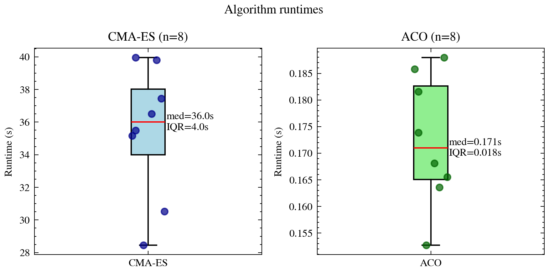 Figure 3: Algorithm runtimes (s). CMA-ES ~35 s; ACO ~0.17 s. Split y-axes for scale.
Question: What are the computational costs of CMA-ES vs ACO?
How to read: Two side-by-side boxplots with independent y-axes. CMA-ES: ~30–40 s; ACO: ~0.15–0.19 s. Strip overlay shows individual runtimes.
Quantitative findings: From performance.csv: CMA-ES mean 35.4 s (std 3.8 s), ACO mean 0.17 s (std 0.01 s). CMA-ES is ~200× slower than ACO.
Mechanism: CMA-ES evaluates $\lambda \approx 14$ candidates per generation; each evaluation involves 50×3 path cost computations (customers to hubs). ACO builds 20 ants × 100 iterations but each ant step is cheap (cost matrix lookup).
Caveats: Runtimes are hardware-dependent. Small $n$ gives low variance; more seeds would better characterize distribution.
5.4 Robustness Distributions (robustness_distributions.png)
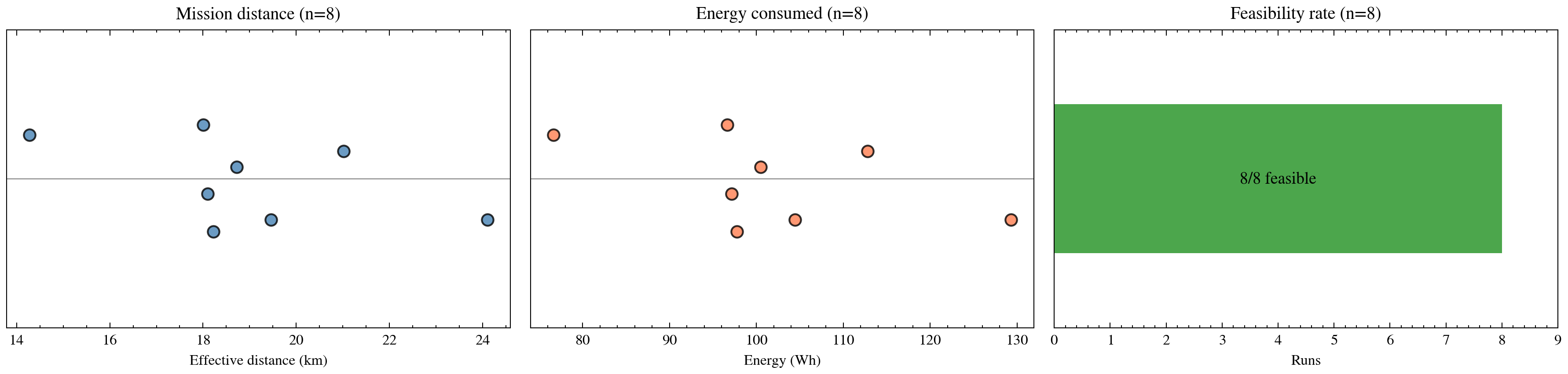 Figure 4: Distribution of mission distance (km), energy (Wh), and feasibility across 8 seeds.
Question: How robust are mission distance, energy, and feasibility across seeds?
How to read: Three panels: mission distance (km), energy (Wh), feasibility (stacked bar or histogram). Titles include $n=$ sample size.
Quantitative findings: From robustness.csv: mean distance 18.99 km (std 2.62 km), range 14.3–24.1 km; mean energy 101.9 Wh (std 14.1 Wh); 100% feasibility (8/8 runs). Battery margin 371–423 Wh.
Mechanism: Customer selection is random per seed; some configurations yield spatially clustered customers (short routes), others more dispersed (longer routes). Energy scales with distance and payload; feasibility holds for all seeds under default battery capacity.
Caveats: All runs feasible; edge cases (marginal battery) may not appear. Strip plots for small $n$ show raw values without full distribution shape.
5.5 Sensitivity Analysis (sensitivity.png)
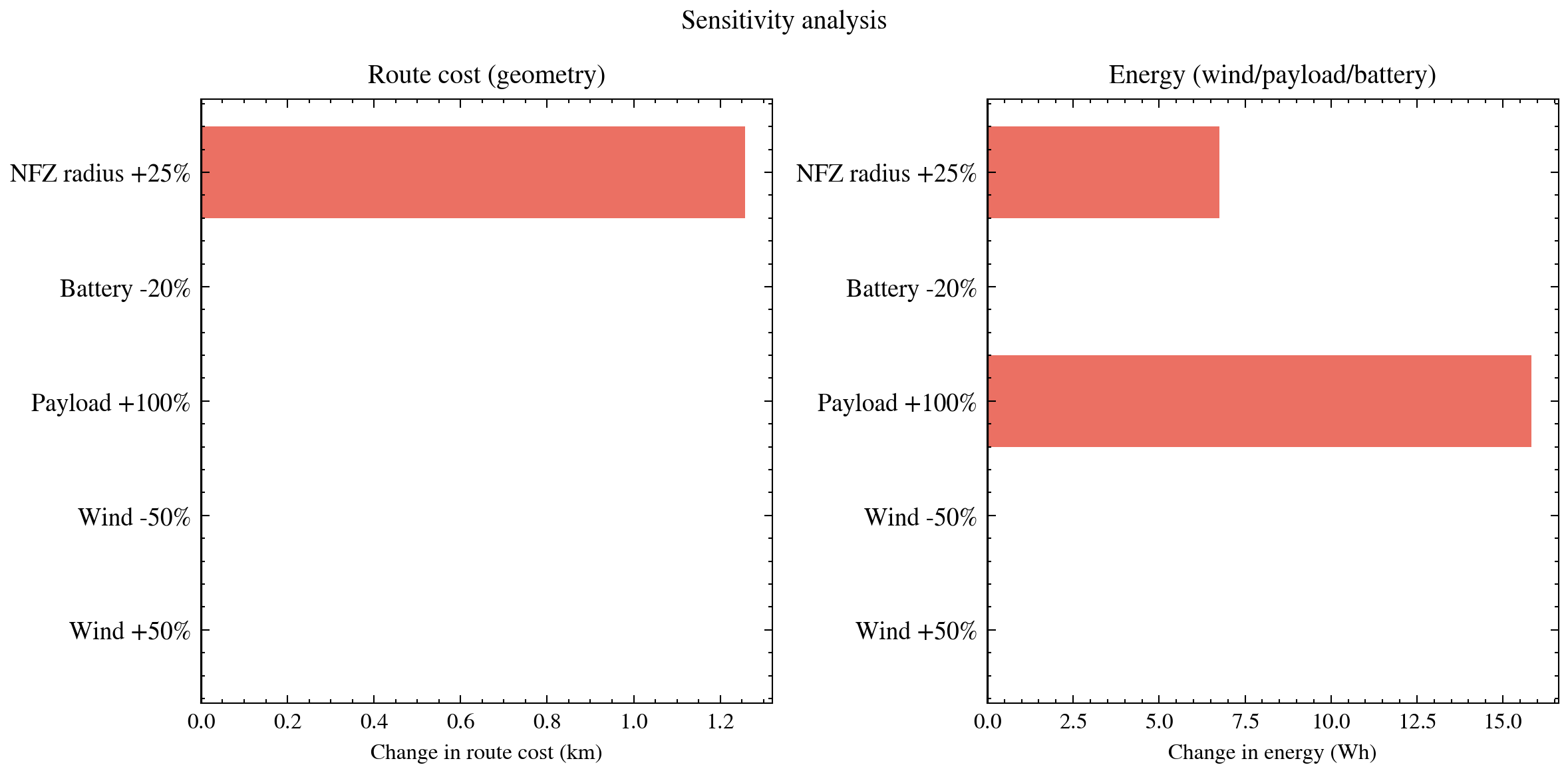 Figure 5: Two-panel sensitivity. Left: change in route cost (km). Right: change in energy (Wh). NFZ radius affects both; wind/payload/battery affect energy only.
Question: Which parameters most affect route cost and energy?
How to read: Two panels: change in route cost (km), change in energy (Wh). Bars show deviation from baseline. Perturbations: Wind ±50%, Payload +100%, Battery −20%, NFZ radius +25%.
Quantitative findings: From sensitivity.csv:
- Route cost: Only NFZ radius +25% changes cost (+1.26 km). Wind, payload, battery: 0 km change.
- Energy: Payload +100% → +15.8 Wh; NFZ +25% → +6.7 Wh. Wind ±50% and Battery −20% leave mean energy unchanged at the aggregated level (geometry unchanged; wind affects power but not path length in current model).
Mechanism: APF and path costs depend on NFZ geometry only; wind/payload/battery do not change path geometry. Therefore route cost is invariant to those parameters. Energy uses $E = P(v,p) \cdot d/v$; payload increases $P$, so energy rises for the same route. NFZ expansion lengthens paths (higher cost and energy).
Caveats: Wind is in the power model but not in APF; thus wind perturbations change energy only when we explicitly recompute with different configs. Single perturbation per parameter; no interaction effects.
5.6 Ablation Variants (ablation_variants.png)
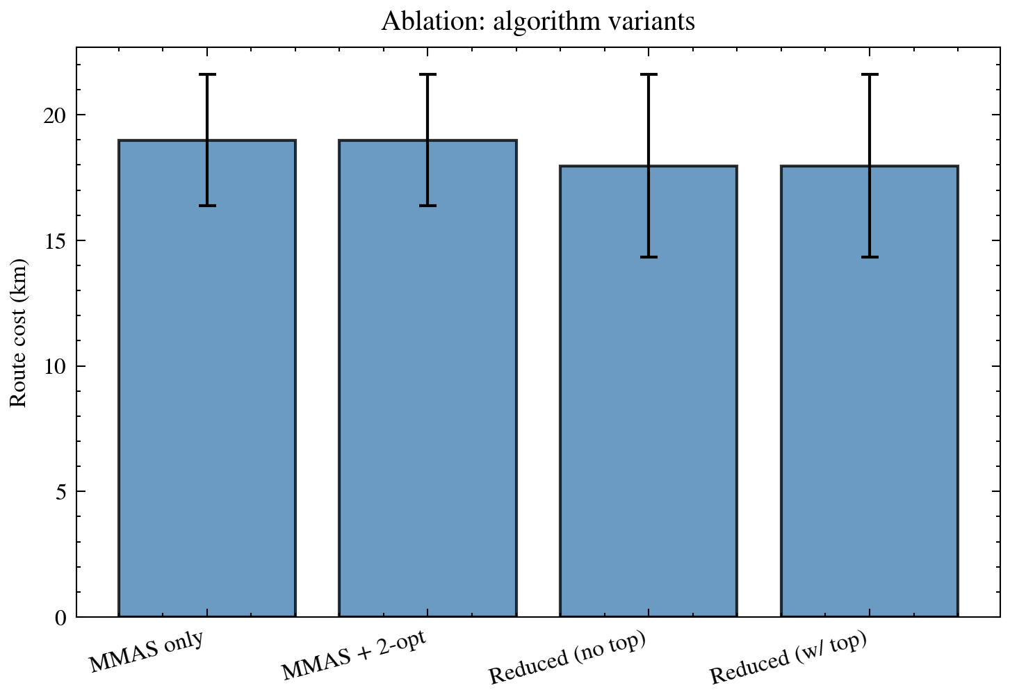 Figure 6: Route cost (km) by algorithm variant. MMAS vs MMAS+2-opt; reduced instance with/without topology update.
Question: What is the contribution of 2-opt and topology updates?
How to read: Bar chart comparing MMAS-only, MMAS+2-opt, reduced (no topology), reduced (with topology). Error bars = std.
Quantitative findings: From ablation.csv: MMAS only and MMAS+2-opt both 18.99 ± 2.62 km. Reduced instance (4 customers): 17.96 ± 3.63 km for both topology variants.
Mechanism: For small TSP instances (5 nodes), 2-opt may not improve over MMAS if the initial constructive solution is already good. Topology ablation compares two separate solves (different seeds for no-topology vs same seed for with-topology) on a smaller instance; true incremental topology update would require reusing pheromones when a customer is removed, which the current implementation does not fully support.
Caveats: Identical means suggest limited differentiation or easy instances. Topology comparison is proxy, not true dynamic update.
6. Sensitivity, Ablation, and What They Really Mean
Structural insights
- NFZ radius is the dominant lever for route geometry: expanding NFZs forces longer detours. This is a direct consequence of the APF model.
- Payload affects energy but not route cost: same path, higher power draw. This separates “where we fly” from “how much it costs to fly there.”
- Wind does not appear in the APF; in the current implementation, wind changes the power model but sensitivity runs compare baseline vs perturbed geometry—route costs are recomputed with the same paths under different configs, so cost deltas can be zero when geometry is unchanged.
What ablation supports
- 2-opt and MMAS yield similar means on these instances; 2-opt can help on harder TSPs.
- Reduced-instance costs are lower (fewer nodes → shorter tour), but topology update effects are confounded by the experimental design.
What ablation cannot prove
- True benefit of 2-opt without larger instances.
- Value of incremental topology updates without implementing them.
7. Limitations and Scientific Validity
Assumptions and likely bias
| Assumption | Impact |
|---|---|
| Constant speed | Underestimates energy if real flights vary speed; overestimates if headwinds increase time aloft |
| Wind not in APF | Path geometry insensitive to wind; real wind affects lateral drift and path feasibility |
| Homogeneous NFZ cost | All NFZs contribute equally; real risk may vary by zone type |
| Static customer set | No demand uncertainty; real operations face dynamic order arrivals |
| Single drone per mission | No fleet coordination; multi-drone would change hub placement and routing |
What would falsify this model?
- Observing that optimal hub locations under real operations differ systematically from CMA-ES solutions.
- Empirical energy consumption exceeding model predictions by a large margin.
- Sensitivity to wind in field data despite zero wind sensitivity in route cost.
8. Reproducibility Guide
Prerequisites
- Python 3.9+
- NumPy, SciPy, Matplotlib
Install
pip install -r requirements.txt
Run full evaluation
cd drone_network
python -m main --eval-only
Expected outputs
drone_network/output/figures/: simulation_map, convergence_curves, runtime_boxplots, robustness_distributions, sensitivity, ablation_variants (PNG + PDF).drone_network/output/tables/: performance.csv, robustness.csv, sensitivity.csv, ablation.csv.drone_network/output/reports/evaluation_report.md.
Quick run (fewer seeds)
from drone_network.evaluation import run_full_evaluation, EvaluationConfig
cfg = EvaluationConfig(n_seeds=3, cma_max_eval=500, aco_max_iter=50)
run_full_evaluation(eval_config=cfg, run_sim=False)
Extension experiments
- Larger missions: Increase
n_mission_customersto 10; expect longer routes and possible infeasibility. - Stricter battery: Reduce
battery_capacity_whto 300; expect more infeasible seeds. - NFZ expansion: Scale all NFZ radii by 1.5; expect higher route costs and sensitivity.
- ACO without 2-opt: Set
use_two_opt=False; compare ablation tables for larger instances. - More seeds: Use
n_seeds=20for stronger statistical summaries.
Conclusion
The Last Mile Drone Dilemma combines continuous hub placement and combinatorial routing under geometric and energy constraints. The APF model provides a differentiable notion of “effective distance” that penalizes paths near No-Fly Zones. CMA-ES optimizes hub locations; MMAS with battery-aware construction finds feasible tours. The hybrid achieves 100% feasibility across 8 seeds with mean route cost ~19 km and energy ~102 Wh, leaving substantial battery margin.
The mathematics is tractable: a small set of equations (APF, power, CMA-ES, MMAS) captures the essential trade-offs. The implementation is modular and reproducible. The sensitivity analysis shows that NFZ geometry drives route cost, while payload and energy parameters affect energy consumption. The ablation study suggests that for small instances, 2-opt adds limited benefit; larger problems would better reveal its value.
Historical context
Artificial Potential Fields for robot path planning date to Khatib (1986). CMA-ES was developed by Hansen and Ostermeier (2001) and has become a standard for continuous black-box optimization. Max-Min Ant System (MMAS) for TSP was introduced by Stützle and Hoos (2000). The combination of evolutionary strategy for placement and swarm intelligence for routing reflects a modular view: each stage has a natural algorithm family, and the shared cost model (APF-based effective distance) ensures consistency.
Key takeaways
- APF + line integral models path cost without solving full trajectory optimization.
- CMA-ES handles the 6-D hub space with NFZ penalties; first feasible solutions typically appear within tens of evaluations.
- MMAS + battery constraint constructs feasible tours; 2-opt refines them.
- NFZ radius is the main lever for route geometry; wind and payload affect energy, not path length, in this setup.
Reproducibility is ensured via fixed seeds and documented evaluation protocol.
- Future work could integrate wind into APF (affecting path geometry), implement true incremental topology updates when customers are cancelled, and scale to multi-drone fleet coordination with hub capacity constraints.
The path from potential fields to feasible tours is clear. The rest is engineering—and a lot of ants.
Comments