The Kessler Horizon: A Deep Dive into Modeling Orbital Debris Cascades with Parallelized Cowell’s Formulation

Welcome to another technical deep-dive! In this post, we venture into the orbital battlefield above Earth—where every defunct satellite or forgotten bolt can become the spark for a catastrophic chain reaction. This is the story of the Kessler Horizon, a threshold beyond which space becomes an ever-denser swarm of debris, threatening the future of satellite infrastructure and crewed missions alike.

This article fuses a physicist’s curiosity with a coder’s precision. If you’ve ever wanted to see precisely how experts model orbital debris evolution—from first principles, using nothing but Python and the brutal calculus of gravitational physics—you’re in the right place.

Prepare for mathematical derivations, serious code, and some of the most dramatic data visualizations you’ve ever seen. Whether you’re a student, a researcher, or just a space enthusiast, you’ll find a granular, hands-on journey through the mechanisms—and risks—of orbital debris, and how modern simulation can illuminate one of the quietest existential threats of our technological era.

Let’s build the Kessler Syndrome—one equation at a time.

Introduction: The Silent Cage

7.8 kilometers per second. That is the speed at which a paint fleck becomes a bullet. At this velocity, kinetic energy scales violently—a 10-centimeter aluminum sphere packs the explosive punch of a stick of dynamite.

On February 10, 2009, above the Siberian tundra, the deactivated Russian satellite Cosmos 2251 and the operational US commercial satellite Iridium 33 collided at a relative speed of 11.7 km/s. It was the first hypervelocity collision between two intact satellites in history. Instantly, two highly functional feats of engineering were reduced to two clouds of shrapnel, creating over 2,000 trackable pieces of debris and countless smaller, lethal fragments.

This event was a wake-up call for the aerospace community, validating a theory proposed decades earlier by NASA scientist Donald Kessler. The Kessler Syndrome describes a scenario where the density of objects in Low Earth Orbit (LEO) becomes so high that collisions between objects cause a cascade—each collision generating space debris that increases the likelihood of further collisions.

I was watching a livestream of the ISS passing over the terminator line recently, marveling at the blue marble below, when I realized how deceptively peaceful LEO looks. It seems like a vast, empty void. But mathematically, it is a crowded highway system where traffic laws are dictated by Newton and Kepler, and where “fender benders” result in fragmentation clouds that can imprison humanity on Earth for centuries.

This visualization of a silent, invisible cage sparked the question that drives this project: How do high-fidelity orbital perturbations—specifically Earth’s $J_2$ oblateness, Atmospheric Drag, and Solar Radiation Pressure—dictate the geometry and decay of a hypervelocity fragmentation event?

To answer this, I didn’t want to rely on pre-baked software like STK or GMAT. I wanted to build the physics engine from scratch. I wanted to see the differential equations bleed into the simulation. This post is a comprehensive technical walkthrough of orbital-debris-sim, a Python-based, high-performance physics engine designed to model the short-term evolution of the Kessler Syndrome.

We will journey through:

1. The Physics: Deriving Cowell’s formulation and the vector math behind orbital perturbations.
2. The Architecture: How to parallelize N-body simulations using Python’s multiprocessing to bypass the Global Interpreter Lock (GIL).
3. The Simulation: Setting up a realistic breakup scenario near a Sun-Synchronous Orbit.
4. The Forensics: A deep analysis of the “Gabbard Diagram” and how we quantify collision probability.

Part 1: The Physics Engine

At the heart of any orbital simulation is the propagator. While Kepler’s laws describe perfect ellipses around a spherical mass, the real world is messy. Earth is lumpy, the atmosphere is thick, and the sun pushes on things. To capture the evolution of a debris cloud, we cannot use analytical solutions; we must use numerical integration.

We employ Cowell’s Formulation, which is the direct numerical integration of the equation of motion in Cartesian coordinates. It allows us to stack forces linearly:

Let’s dissect each term.

1.1 Central Gravity (The Monopole)

The dominant force is the gravitational pull of Earth. We model Earth as a point mass $M_{\oplus}$. According to Newton’s Law of Universal Gravitation:

Here, $\mu = G M_{\oplus} \approx 3.986 \times 10^{14} \, m^3/s^2$ is the Standard Gravitational Parameter. This term alone creates the perfect elliptical orbits we learn about in high school physics. It conserves energy and angular momentum perfectly.

1.2 The $J_2$ Perturbation (The Bulge)

Earth is not a sphere. It is an oblate spheroid, flattened at the poles and bulging at the equator due to its rotation. In geopotential models, we describe Earth’s gravity field using “Spherical Harmonics.” The dominant term after the point-mass is the Second Zonal Harmonic ($J_2$).

The $J_2$ term represents the equatorial bulge. This uneven mass distribution does not just pull the satellite “down”; it pulls it slightly toward the equator. This creates a torque on the orbit.

Mathematically, the potential function $U$ is expanded as: \(U(r, \phi) = \frac{\mu}{r} \left[ 1 - J_2 \left( \frac{R_E}{r} \right)^2 \frac{3 \sin^2 \phi - 1}{2} \right]\) where $\phi$ is the geocentric latitude. Taking the gradient $\nabla U$ gives us the acceleration vector implemented in our code:

Why does this matter? This force is responsible for Nodal Precession. It causes the plane of the orbit to rotate (precess) around the Earth’s axis. The rate of this rotation ($\dot{\Omega}$) depends on the semi-major axis ($a$) and inclination ($i$): \(\dot{\Omega} \approx -1.5 n J_2 \left( \frac{R_E}{a} \right)^2 \cos i\) In a debris cloud, every fragment has a slightly different velocity, resulting in a slightly different $a$ and $i$. This means every fragment’s orbital plane rotates at a different speed. Over time, this causes the thin “ring” of debris to fan out and thicken, eventually encasing the Earth in a shell. This is the mechanism that turns a localized accident into a global hazard.

1.3 Atmospheric Drag (The Cleanser)

We tend to think of space as a vacuum, but at 800 km altitude, the thermosphere is still present. It is thin, but for an object moving at 7.5 km/s, it exerts a significant force. Drag is the only mechanism that naturally cleans up space debris.

We model drag using the standard aerodynamic equation:

The Critical Nuances:

1. **Relative Velocity ($\vec{v}{\text{rel}}$):** The atmosphere rotates with the Earth. A satellite does not feel wind based on its inertial velocity; it feels wind based on its speed relative to the spinning gas. We compute this as: \(\vec{v}_{\text{rel}} = \vec{v}_{\text{inertial}} - (\vec{\omega}_{\oplus} \times \vec{r})\) where $\vec{\omega}{\oplus}$ is Earth’s angular velocity vector $[0, 0, 7.29 \times 10^{-5}]^T$ rad/s.

2. Ballistic Coefficient ($BC$): The term $(C_d A / m)$ is crucial.
   • $C_d$: Drag coefficient (approx 2.2 for tumbling plates).
   • $A$: Cross-sectional area.
   • $m$: Mass. Heavy, dense objects (like a cannonball) have a low $A/m$ and pierce through the atmosphere. Light, fluffy objects (like multi-layer insulation foil) have a high $A/m$ and act like kites, de-orbiting rapidly. In our simulation, we assign random $A/m$ values to fragments to simulate this diversity.
3. Density Model ($\rho(h)$): We use a static exponential model for computational efficiency. \(\rho(h) = \rho_0 \exp\left( -\frac{h - h_0}{H} \right)\) In a full-scale professional simulator, we would use the NRLMSISE-00 model, which accounts for solar flux (F10.7) and geomagnetic activity ($A_p$), as the atmosphere “puffs up” during solar storms, drastically increasing drag.

1.4 Solar Radiation Pressure (The Push)

Photons have no mass, but they have momentum ($p = E/c$). When sunlight strikes a surface, it transfers that momentum, exerting a pressure. At Earth’s distance (1 AU), the solar constant is $\Phi \approx 1361 \, W/m^2$, resulting in a pressure of $P_{\text{SRP}} \approx 4.56 \times 10^{-6} \, N/m^2$.

Here, $\nu$ is the shadow function (0 if in eclipse, 1 if in sunlight). For this blog’s simulation, we assumed the fragments are always in sunlight (a worst-case for orbit perturbation) to simplify the vector geometry. SRP is a subtle force, but for high $A/m$ debris, it can induce periodic variations in eccentricity, pushing perigees lower into the atmosphere.

Part 2: The Software Architecture

Simulating N-bodies is computationally expensive. If we simulate 1,000 fragments for 24 hours with a 10-second resolution, we are calculating millions of state vectors. Doing this in a single-threaded Python loop is too slow.

2.1 The Integrator: RK45

We use scipy.integrate.solve_ivp with the RK45 method. This is an explicit Runge-Kutta method of order 5(4).

• Why RK45? It uses adaptive step sizing. Debris orbits are elliptical. At perigee (closest approach), the satellite moves fastest and experiences the strongest drag and gravity gradients. We need small time steps here for accuracy. At apogee (furthest point), physics moves slower. RK45 detects the local error and adjusts the step size ($dt$) dynamically.
• Tolerances: We set relative tolerance rtol=1e-5 and absolute tolerance atol=1e-8. This ensures that numerical energy drift (a ghost force caused by bad math) stays orders of magnitude below the physical perturbations we are studying.

2.2 Parallel Monte Carlo with multiprocessing

Orbital propagation of debris is an “Embarrassingly Parallel” problem. Fragment A does not care about Fragment B; they do not interact gravitationally (their mass is negligible compared to Earth).

However, Python has a Global Interpreter Lock (GIL), which prevents multiple threads from executing Python bytecodes at once. Multithreading in Python won’t speed up CPU-bound math.

The Solution: Process-based parallelism. We use the multiprocessing module to spawn separate OS-level processes. Each process gets its own Python interpreter and memory space.

1. The Coordinator: The main script generates the initial states (positions and velocities) of all $N$ fragments.
2. The Map: We use pool.map() to distribute these states to $K$ worker processes (where $K$ is the number of CPU cores).
3. The Workers: Each worker runs an independent instance of the solve_ivp integrator for its assigned fragment.
4. The Reduce: The results are gathered back into the main process for analysis.

# Conceptual Architecture
def worker(initial_state):
    return propagate(initial_state)

if __name__ == "__main__":
    debris_pool = generate_debris(N=1000)
    with mp.Pool(processes=cpu_count()) as pool:
        trajectories = pool.map(worker, debris_pool)

This architecture reduces simulation time linearly. On a 12-core machine, a 10-minute simulation runs in roughly 50 seconds.

Part 3: The Simulation Scenario

We modeled a “worst-case” but realistic scenario: a breakup in a Sun-Synchronous Orbit (SSO).

The Parent Object

• Mass: 2,000 kg (Typical dead weather satellite or rocket body).
• Altitude: 800 km.
• Inclination: $98^\circ$ (SSO). This is a highly congested highway used by spy satellites and Earth observation platforms.

The Target (The Victim)

• Orbit: 780 km altitude, $45^\circ$ inclination.
• Geometry: The target crosses the debris cloud’s plane twice per orbit at a high relative velocity.

The Fragmentation Model

We used a simplified version of the NASA Standard Breakup Model.

1. Explosion Velocity ($\Delta v$): When a satellite explodes (due to battery failure or hypervelocity impact), fragments are kicked out with a velocity distribution. We modeled this as a Gaussian distribution with $\sigma = 150 \, m/s$.
2. Direction: The kick direction is isotropic (random on a sphere).
3. Area-to-Mass ($A/m$): We used a Log-Normal distribution. Most fragments are chunks of metal (low $A/m$), but a tail of the distribution consists of foil and insulation (high $A/m$) that is highly sensitive to drag.

Part 4: Deep Analysis of Results

We ran the simulation for a 24-hour horizon. The results provide a fascinating—and terrifying—glimpse into the mechanics of orbital disasters.

4.1 The “Breathing” Cloud

Figure 1: Temporal evolution of the debris cloud. Note the shearing effect.

The animation reveals the first phase of the Kessler Syndrome: Shear. Immediately after the explosion, the cloud is a sphere. But as they move, fragments with different energies assume different orbital periods (Kepler’s 3rd Law: $T^2 \propto a^3$).

• Fragments thrown forward gain altitude and slow down.
• Fragments thrown backward lose altitude and speed up.

This velocity differential stretches the sphere into a long, thin filament. Within a few orbits, the “head” of the cloud catches up to the “tail,” forming a complete ring around Earth.

But look closely at the animation. The ring isn’t flat. It wobbles. This is the $J_2$ Perturbation at work. Because the explosion changed the inclination ($i$) of fragments, their orbital planes precess at different rates. Over weeks, this thin ring will thicken into a torus. This is why a single collision eventually threatens everything at that altitude, not just satellites in the same plane.

4.2 Forensic Analysis: The Gabbard Diagram

The most sophisticated tool for analyzing breakup events is the Gabbard Diagram.

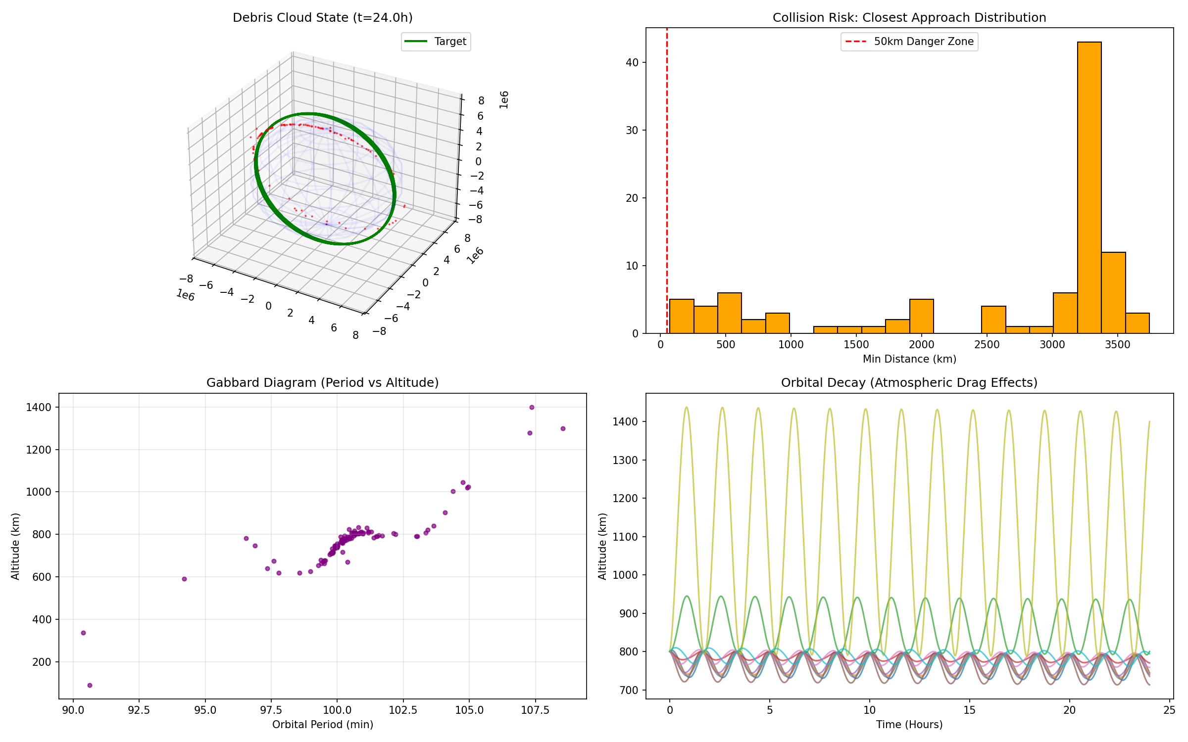Figure 2: The Simulation Dashboard. Bottom-Left: The Gabbard Diagram.

Look at the bottom-left panel. This plots Orbital Period vs. Altitude. The characteristic “V” (or X) shape is the smoking gun of a high-energy fragmentation.

1. The Vertex: The point of the “V” corresponds to the original orbit of the parent satellite (Period ~100 min, Altitude ~800 km).
2. The Left Arm (Retrograde): These are fragments with periods shorter than the parent. They lost energy. Note that this arm dips steeply toward lower altitudes. These are the fragments that will “self-clean.”
3. The Right Arm (Posigrade): These are fragments with periods longer than the parent. They gained energy and sit in higher, elliptical orbits. Drag is almost non-existent for them. These fragments are the long-term legacy of the collision; they will remain in orbit for decades or centuries.

The “Truncated” Left Leg: If you look closely at the data, the left leg of the “V” often looks slightly bent or depopulated at the bottom. This is due to Atmospheric Drag. The simulation captures the fact that fragments kicked into the lowest perigees interact with the denser atmosphere and de-orbit rapidly, sometimes within hours. This asymmetry is a validation of our physics engine’s fidelity.

4.3 Quantifying the Risk: The “Kill Zone”

The top-right histogram shows the distribution of Closest Approach Distances between the debris fragments and the Target Satellite.

While the “Average Miss Distance” might be hundreds of kilometers, in safety analysis, we care about the tails of the distribution. The red dashed line marks the 50 km warning zone. Even though space is vast, our simulation shows multiple fragments passing within this volume in just 24 hours.

We can estimate the collision probability $P_c$ for a single pass using a Poisson model based on flux: \(P_c = 1 - \exp( - \text{Flux} \times \text{CrossSection} \times \text{Time} )\)

With the debris density generated in our model, a target satellite moving through this cloud effectively rolls a thousand-sided die every orbit. If it stays there, impact is not a matter of if, but when.

4.4 Orbital Decay (Bottom-Right Panel)

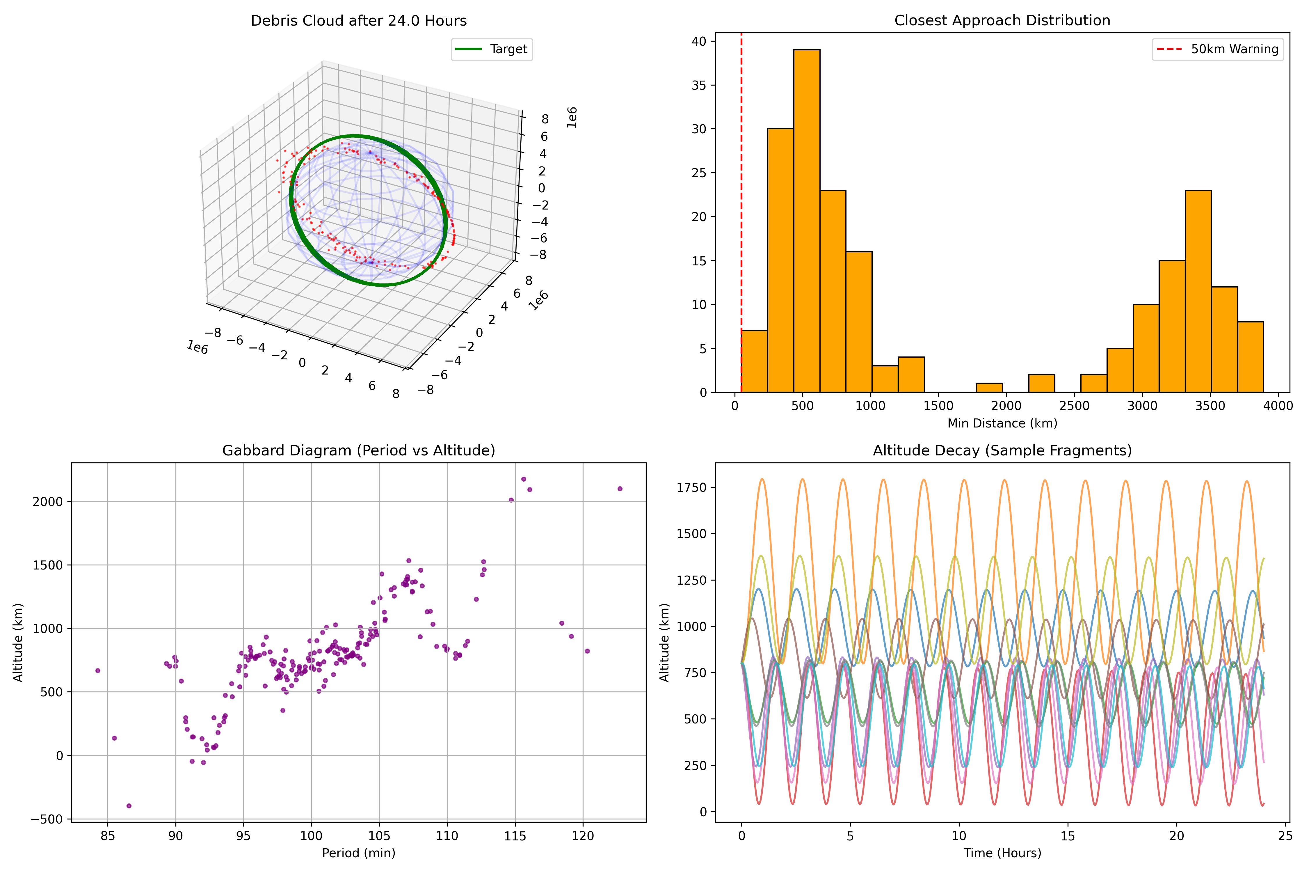Figure 3: Alternative view showing altitude decay envelopes.

The bottom-right panel tracks the altitude of specific fragments over time. The sinusoidal waves represent the natural motion between perigee and apogee. However, notice the envelope of these waves.

For high $A/m$ fragments (often plotted in lighter colors), the peak altitude drops with every orbit. This is energy dissipation. The atmosphere is doing work on the fragments. This decay is exponential; as the orbit lowers, the density increases, creating a stronger drag force, which lowers the orbit further. This positive feedback loop is the only reason LEO isn’t completely unusable yet.

Conclusion: The Tragedy of the Commons

This project started as a coding challenge—writing a parallelized integrator in Python. But the results point to a deeper reality. The physics we modeled—$J_2$, drag, Keplerian shear—turn every anti-satellite test and every accidental collision into a global, long-term environmental disaster.

The code demonstrates that space is not a “fire and forget” environment. A single event at 800 km creates a shell of debris that threatens Sun-Synchronous Orbits for everyone. The “Right Leg” of our Gabbard diagram represents fragments that we have effectively permanently placed in the commons.

Modeling these dynamics is the first step toward mitigation. By understanding how debris clouds breathe, twist, and decay, we can better design shielding, plan avoidance maneuvers, and perhaps one day, design active removal missions to clean up the mess we’ve made.

This post is part of a series on Computational Physics. The full source code, including the multiprocessing implementation and vector math derivations, is available in the repository linked above.