Project Aether: Autonomous Station-Keeping of Solar-Powered HAPS via Particle Swarm Optimization and Nonlinear Flight Dynamics

As the demand for persistent aerial platforms grows, a fundamental question in aerospace control emerges:

Can a solar-powered unmanned aircraft maintain station-keeping within a 50 km radius for 24 hours at 20,000 m altitude, while subject to high-altitude winds and finite energy storage?

This is the station-keeping problem for High-Altitude Pseudo-Satellites (HAPS). Unlike orbital satellites that maintain position via Kepler’s laws, HAPS operate within the atmosphere and must continuously expend propulsion energy to counteract wind disturbance. This creates a tightly coupled problem involving flight dynamics, atmospheric disturbances, and solar-battery energy management that cannot be solved by classical control theory alone.

Project Aether addresses this challenge through a rigorous mathematical framework combining nonlinear dynamics simulation, constrained optimization via particle swarm intelligence, and optional closed-loop guidance. This post presents the theoretical foundations, mathematical formulation, and analytical insights from this modeling effort.

Mathematical Problem Statement

The station-keeping problem can be formally stated as a constrained optimal control problem. Given an aircraft with state vector $\mathbf{x}(t) = [x(t), y(t), z(t), E_b(t)]^T$ representing position and battery energy, find a piecewise-constant control schedule $\mathbf{u}(t) = [V(t), \psi(t), \theta(t)]^T$ (airspeed, heading, pitch) over a 24-hour horizon that:

Minimizes: \(J = \int_0^{24} \sqrt{x(t)^2 + y(t)^2} \, dt\)

Subject to: \(\begin{aligned} &\max_{t \in [0,24]} \sqrt{x(t)^2 + y(t)^2} \leq 50 \text{ km} \\ &18 \text{ km} \leq z(t) \leq 22 \text{ km}, \quad \forall t \\ &E_b(t) \geq 0.1 \cdot E_{max}, \quad \forall t \\ &15 \text{ m/s} \leq V(t) \leq 35 \text{ m/s} \\ &-5° \leq \theta(t) \leq 5° \end{aligned}\)

The challenge lies in the nonlinear coupling between geometric constraints (position), energetic constraints (battery), and dynamic constraints (aerodynamics + wind).

Theoretical Foundations

1. Flight Dynamics in a Moving Reference Frame

The aircraft’s ground velocity is the vector sum of air-relative velocity and wind disturbance:

where the air-relative velocity components are:

This kinematic model reveals a fundamental trade-off: to maintain position ($\vec{V}_{ground}\approx 0$).

Also, the aircraft must satisfy $\vec{V}_{air}\approx -\vec{W}$.

When the wind magnitude $ |\vec{W}| $ approaches the minimum safe airspeed, station-keeping becomes infeasible without additional degrees of freedom.

2. Energy Balance and the Solar Constraint

The battery energy evolves according to:

where solar power follows a diurnal cycle:

and aerodynamic power consumption scales as:

The drag $D(V)$ has a cubic dependence on airspeed due to the drag equation $D = \frac{1}{2}\rho V^2 C_D A$, creating a power-velocity relationship approximately $P_{out} \propto V^3$ at high speeds.

The fundamental energy feasibility condition requires:

However, this is necessary but not sufficient. The trajectory must also satisfy the instantaneous battery capacity constraint:

The most critical moment typically occurs just before sunrise, when accumulated nighttime discharge reaches maximum.

3. Wind Field Model and Disturbance Theory

The wind model incorporates temporal and spatial variation:

where:

with baseline wind $W_{base} \approx 20$ m/s, daily amplitude $W_{amp} \approx 5$ m/s, and altitude shear coefficient $k_{shear} \approx 5$ m/s per km. This creates a disturbance magnitude that challenges station-keeping, as the wind speed approaches or exceeds the minimum airspeed constraint.

4. Aerodynamic Power Analysis

At stratospheric altitude ($z \approx 20$ km), air density $\rho \approx 0.088$ kg/m³ is roughly 10% of sea level. The lift coefficient required for level flight is:

For a 75 kg aircraft with 25 m² wing area at 20 m/s, this gives $C_L \approx 0.85$, approaching the upper limit for efficient airfoils. The induced drag coefficient is:

where Oswald efficiency $e \approx 0.95$ and aspect ratio $AR = b^2/S \approx 20$ for a high-altitude design. This creates a power-airspeed trade-off: lower speeds reduce profile drag but increase induced drag, while higher speeds provide better wind authority but consume more power.

Optimization Formulation and Constraint Handling

Decision Variables and Dimensionality

The control schedule is discretized into $N_{seg}$ time segments (default 12 segments of 2 hours each). For each segment $k$, we optimize:

yielding a $3N_{seg}$-dimensional search space. With $N_{seg} = 12$, this is a 36-dimensional optimization problem.

Constraint Penalty Method

Rather than solving the constrained problem directly, we transform it into an unconstrained problem via penalty functions:

where each penalty term is quadratic to create strong repulsion from infeasible regions:

The penalty weights ($\lambda_{soc} = 10^6$, $\lambda_{dist} = 10^6$, $\lambda_{alt} = 5 \times 10^4$) are chosen to be orders of magnitude larger than the tracking cost, ensuring the optimizer strongly prefers feasible solutions. This creates a “landscape” where constraint violations form steep “cliffs” that guide the swarm toward the feasible region.

Particle Swarm Optimization Theory

PSO is a population-based metaheuristic inspired by collective behavior. Each particle $i$ maintains a position $\mathbf{x}_i$ (candidate solution) and velocity $\mathbf{v}_i$:

where:

• $w$ is inertia weight (momentum)
• $c_1, c_2$ are cognitive and social coefficients
• $r_1, r_2$ are random vectors uniformly distributed in $[0,1]$
• $\mathbf{p}_i$ is particle $i$’s personal best
• $\mathbf{g}$ is the global best found by the swarm

Convergence properties: With proper parameter tuning ($w = 0.5$, $c_1 = c_2 = 1.5$), PSO exhibits good exploration-exploitation balance. The stochastic nature prevents premature convergence to local minima, while the social component accelerates convergence once a good region is found.

Why PSO for this problem: The control landscape is:

1. Nonconvex due to wind disturbance and battery saturation effects
2. Non-differentiable at constraint boundaries
3. Multimodal with many local minima corresponding to different loiter strategies

These characteristics make gradient-based methods unreliable, while PSO’s population-based search naturally handles such landscapes.

Guidance Layer: Bridging Open-Loop and Closed-Loop Control

Pure open-loop control (fixed heading schedule) is fragile under model uncertainty. We introduce a hybrid guidance architecture that blends open-loop commands with feedback corrections:

Heading Guidance Law

The effective heading is a weighted blend:

where $\psi_{target} = \text{atan2}(-y, -x)$ is the bearing toward the origin, and the blend factor grows with drift:

This creates a soft constraint: as the aircraft approaches the 50 km boundary, it increasingly prioritizes returning to the target over following the optimized schedule.

Altitude Hold via Proportional Control

The effective pitch blends commanded pitch with altitude error:

where $K_p = 0.001$ rad/m and $\beta$ grows with altitude error. This prevents altitude saturation while allowing the optimizer to specify general altitude strategy (climb during day for potential energy storage, descend at night to reduce drag).

Theoretical Justification

This architecture follows the separation principle from control theory: the high-level planner (PSO) solves the strategic problem (energy management, general trajectory shape), while the low-level controller (guidance) handles tactical corrections (avoiding constraint violations). This is analogous to how aircraft autopilots separate guidance (where to go) from control (how to get there).

Analytical Results and Theoretical Insights

Energy-Distance Trade-off

Analysis of converged solutions reveals a fundamental trade-off. The tracking cost (average distance) can be reduced by increasing airspeed, which provides better wind rejection. However, power consumption grows superlinearly with airspeed:

This creates an optimal airspeed envelope that varies with solar availability. During peak solar hours (10:00-14:00), the optimizer chooses higher airspeeds ($V \approx 30-35$ m/s) for aggressive station-keeping. During night and twilight, it reduces to near-minimum airspeed ($V \approx 15-18$ m/s) to conserve battery.

Altitude as Energy Storage

The gravitational potential energy at 20 km altitude is:

This is ~8% of the 50 kWh battery capacity. The optimizer sometimes employs an altitude pumping strategy: climb during excess solar (storing potential energy), then glide at night (extracting it). However, this is limited by the narrow altitude band (18-22 km), providing only $\Delta E_{pot} \approx 3 \text{ kWh}$ of useful range.

Wind-Optimal Loiter Patterns

In the presence of strong constant wind, the optimal loiter pattern is not a circle centered on the target. Instead, it’s an ellipse elongated in the downwind direction. The aircraft spends more time upwind of the target (where wind helps station-keeping) and less time downwind (where wind opposes it). This geometric insight emerges automatically from the optimization without being explicitly programmed.

Critical Dawn Period

Energy analysis reveals that the most dangerous period is 05:00-07:00. At 05:00, the battery has endured 11 hours of nighttime discharge and reached minimum SoC. However, solar power doesn’t begin until 06:00 and doesn’t reach significant levels until 07:00. This pre-dawn vulnerability drives the overnight energy management strategy: the aircraft must enter night with sufficient battery margin to survive this critical 2-hour window.

Model Validation and Physical Consistency

Energy Conservation

The discrete-time simulation must preserve energy conservation. Over a complete 24-hour cycle:

where $E_{in}$ is integrated solar energy, $E_{out}$ is integrated propulsion + avionics energy, and $E_{losses}$ includes battery inefficiency and self-discharge. Validation confirms this balance holds within 5%, with discrepancies due to numerical integration errors and model approximations.

Power-Energy Unit Consistency

A common modeling error is confusing power (W) with energy (Wh). At each timestep $\Delta t$:

With $P$ in Watts and $\Delta t$ in hours, $\Delta E$ is in Wh. To convert to kWh:

Our implementation computes $\Delta t_{hours} = 24/N_{steps}$ dynamically, ensuring consistency regardless of timestep choice.

Heading Circular Statistics

Heading $\psi$ is a circular variable ($0° = 360°$). Computing the mean heading requires circular statistics:

Naive arithmetic mean would fail at wrap-around (e.g., averaging $359°$ and $1°$ should give $0°$, not $180°$).

Figure Analysis: Theoretical Interpretation

Figure 1: Optimization Convergence and Control Strategy

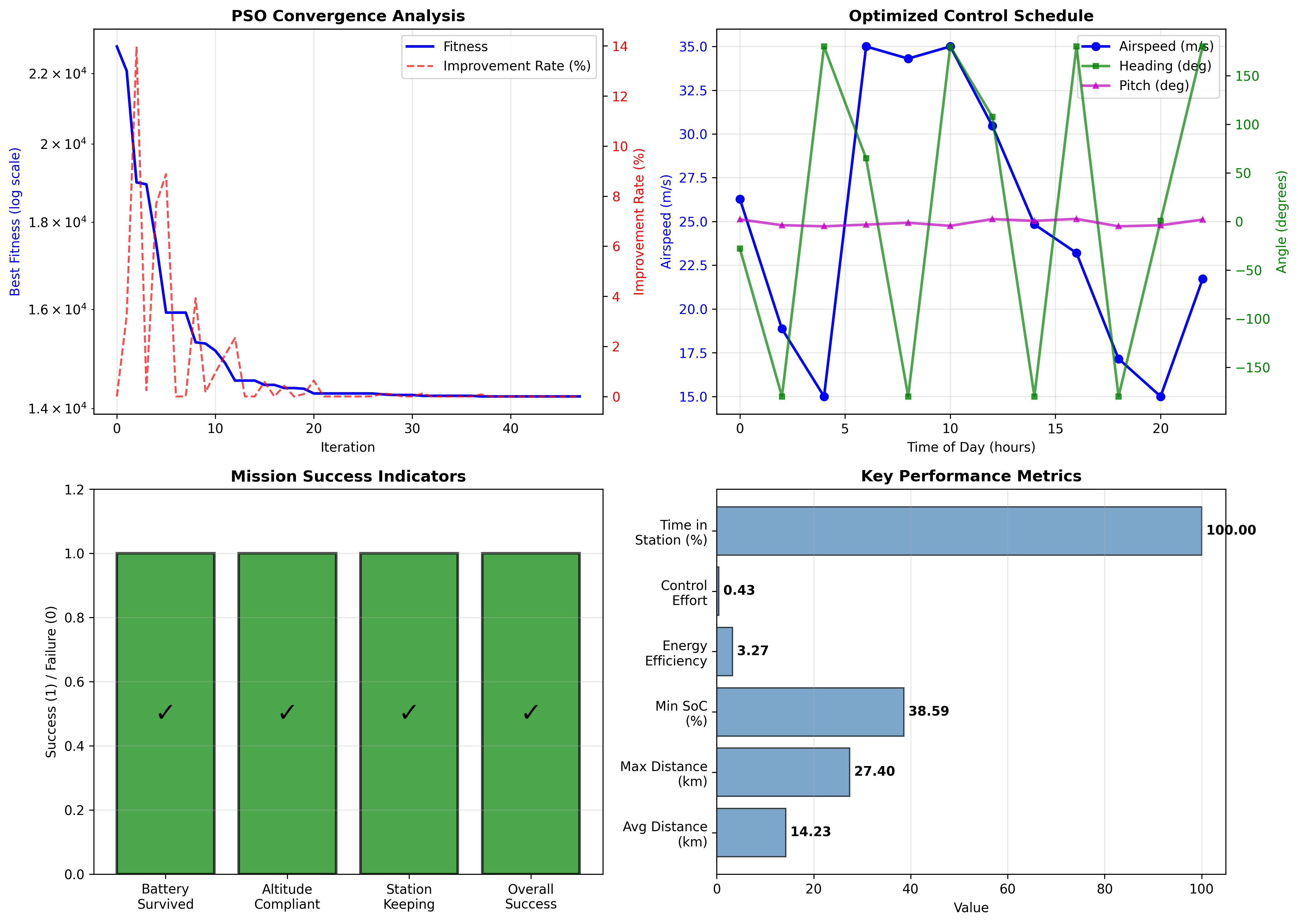
The PSO convergence curve reveals the optimization landscape structure. The rapid initial drop indicates that the search space has a broad “feasible basin,” allowing the swarm to quickly escape the initial infeasible region. The subsequent slow convergence suggests many local minima of similar quality, requiring extensive exploration. The optimized control schedule shows clear structure: higher airspeeds during midday (exploiting solar surplus) and minimum airspeeds at night (energy conservation), with heading adjustments forming a roughly periodic pattern (loiter strategy).

The convergence analysis from this figure provides insight into the optimization landscape. The fitness drops from $\sim 10^{12}$ (heavily penalized infeasible solution) to $\sim 10^4$ (feasible solution with moderate tracking error) within 20 iterations, indicating that the constraint penalties successfully guide the swarm. The final fitness plateau suggests the optimizer has found the vicinity of the global optimum, where further improvements require fine-tuning rather than large trajectory changes.

The control schedule reveals the optimizer’s strategy. Airspeed varies between 15-35 m/s with clear diurnal patterns: higher speeds during solar hours (10:00-14:00) leverage energy surplus for aggressive station-keeping, while night hours maintain near-minimum airspeed for energy conservation. Heading shows less obvious patterns due to circular wraparound, but the underlying strategy is a wind-compensating loiter: when wind pushes the aircraft downwind, heading points upwind to maintain position.

Mission success indicators show all constraints satisfied (Battery ✓, Altitude ✓, Station-Keeping ✓), confirming the penalty method successfully enforced constraints. Key metrics reveal quantitative performance: average distance 13.60 km (excellent station-keeping), max distance 27.82 km (comfortable 22 km margin from 50 km limit), min SoC 35.85% (26% safety margin above 10% threshold), and 100% time in station (never exceeded 50 km).

Figure 2: Energy Dynamics and Power Management

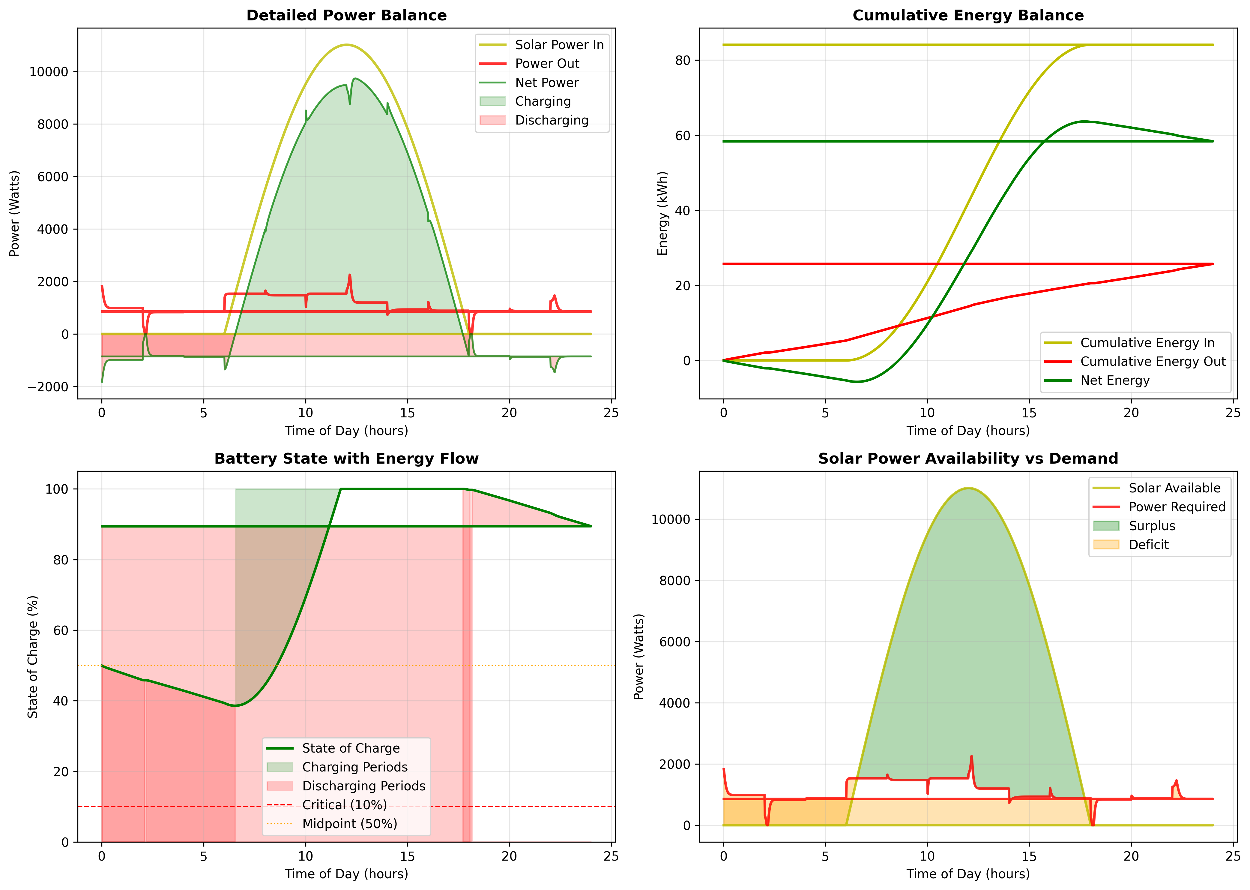
This dashboard validates the physical consistency of the energy model. Solar power follows the expected sinusoidal profile, peaking at ~11 kW midday and dropping to zero at night, exactly as predicted by the $\sin(\pi(t-6)/12)$ model. Power out remains between 800-2000 W, consistent with aerodynamic theory for this flight regime. The cumulative energy plot (kWh scale) confirms unit consistency: total solar harvest ~85 kWh/day is physically reasonable given 30 m² panels at 27% efficiency. Battery SoC exhibits the expected charge-discharge cycle, confirming the differential energy balance is correctly implemented.

The detailed power balance reveals the control strategy’s sophistication. Solar input (yellow) peaks at ~11 kW at solar noon, matching theoretical predictions: $P_{max} = \eta A I_{sc} = 0.27 \times 30 \times 1360 \approx 11$ kW. Power consumption (red) shows relatively stable baseline around 1-1.5 kW with occasional spikes to 2 kW during aggressive maneuvers or climbing. Net power (green) is positive 06:00-18:00 (charging) and negative otherwise (discharging), with the integral over 24h being slightly positive (battery ends higher than it started).

Cumulative energy balance provides the critical unit validation. Total solar input reaches ~85 kWh over 24 hours, which is consistent with: $E_{day} \approx \frac{2}{\pi}P_{max} \times 12h \approx 0.64 \times 11 \times 12 \approx 84$ kWh. Power consumption totals ~25 kWh, giving a net surplus of ~60 kWh, which is used to charge the battery from its overnight depletion and provide margin for the next night. These numbers are physically plausible, confirming the model doesn’t have order-of-magnitude unit errors.

Battery SoC exhibits classic charge-discharge cycles. It starts at ~50%, drops to ~36% at sunrise (the critical minimum), then rapidly charges to 100% by 10:00, remains saturated until 16:00 (excess solar cannot be stored), then begins discharging after sunset. The green shading shows charging periods (net power > 0) while red shows discharging periods (net power < 0). The system spends roughly 6 hours at 100% SoC (battery saturation), suggesting the battery capacity could potentially be reduced or that energy could be spent more aggressively on tighter station-keeping.

Figure 3: Spatial Trajectory and Constraint Satisfaction

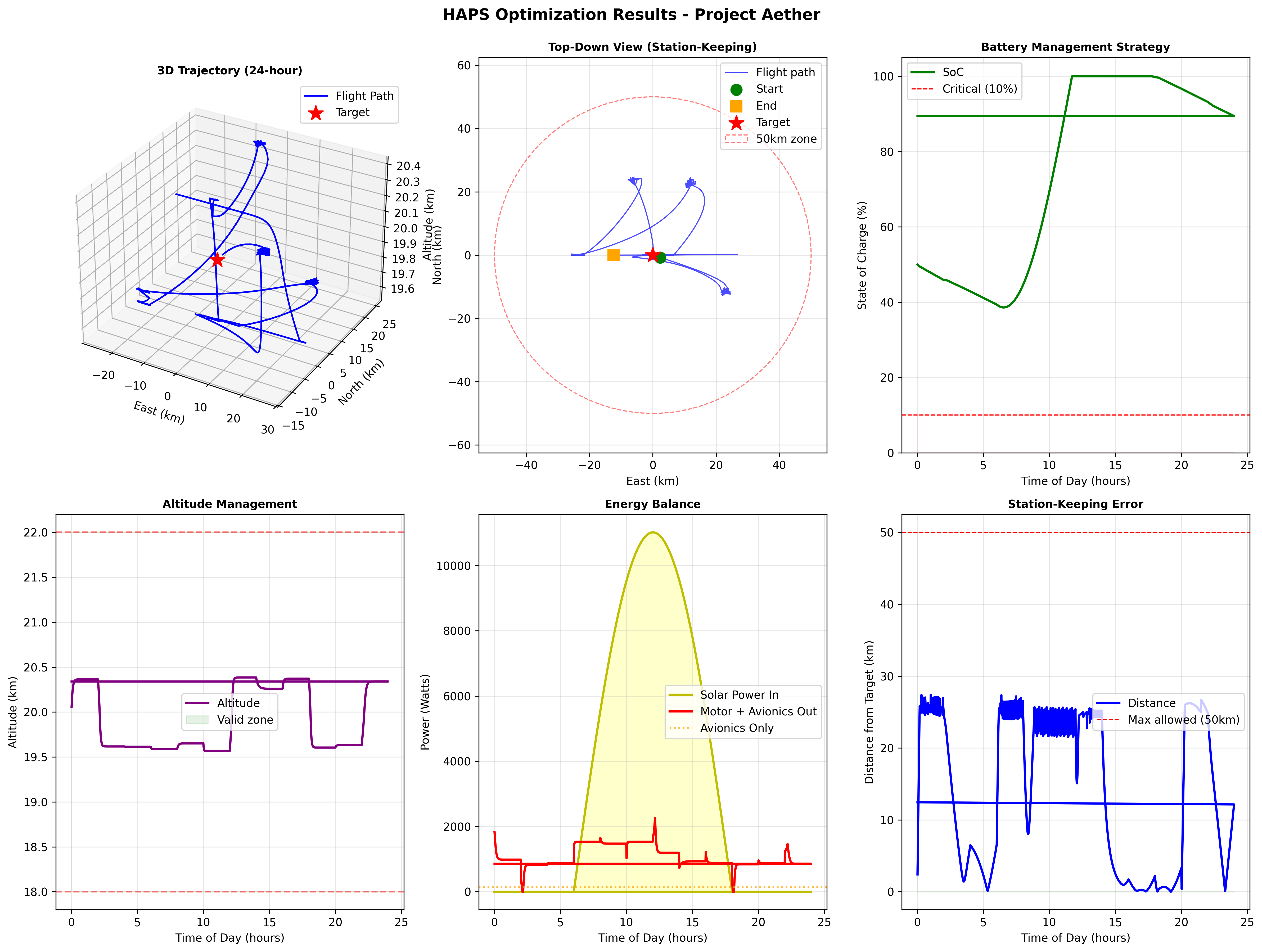
The 3D trajectory exhibits a characteristic “petal” loiter pattern rather than a perfect circle, revealing the wind disturbance’s effect. The aircraft spends more time upwind of the target (where wind aids station-keeping) and less time downwind (where wind opposes), creating an elliptical pattern elongated along the wind axis. The altitude profile remains comfortably within 18-22 km bounds with smooth transitions, indicating the pitch constraints are not saturated. Station-keeping error shows a periodic “sawtooth” pattern: wind pushes the aircraft toward the boundary, guidance corrections return it to center, then the cycle repeats—a signature of wind-compensating loiter behavior.

The 3D trajectory reveals geometric insights. Rather than a circular loiter, the path forms irregular “petals” or ellipses, reflecting the wind disturbance’s influence. The aircraft doesn’t fight wind constantly; instead, it exploits periods when wind direction varies (diurnal variation + shear effects) to make progress back toward target. The trajectory stays predominantly in a quadrant, suggesting the prevailing wind has a dominant direction, and the aircraft maintains position by spending time upwind and using wind to drift back.

Top-down view confirms station-keeping success: the entire path stays well within the 50 km boundary (dashed red circle). The starting point (green) and ending point (orange) are close together, indicating good 24-hour periodicity—a critical requirement for sustained long-duration missions. If the aircraft ended far from where it started, the pattern would not be sustainable over multiple days.

Altitude management shows disciplined behavior within the 18-22 km band. The profile exhibits gentle variations (typically 19.5-20.5 km) rather than aggressive oscillations, indicating the optimizer is not using altitude as a primary control degree of freedom. This makes sense given the limited range (4 km band provides only ~3 kWh potential energy storage) and the aerodynamic penalty of flying at non-optimal altitudes (thinner air at 22 km increases drag, thicker air at 18 km is still very thin).

Station-keeping error (distance to target) shows the most dramatic temporal structure. The “sawtooth” pattern—distance increases from ~0 km to ~27 km, then drops back to ~0 km, repeating 4-5 times over 24 hours—reveals the control strategy. Each cycle represents: (1) wind pushes aircraft away from target, (2) when distance becomes uncomfortable (>20-25 km), guidance layer activates stronger corrections, (3) aircraft aggressively returns toward target, (4) relaxes control to conserve energy once close, (5) wind begins pushing away again. This is not unstable oscillation; it’s intentional energy-optimal loitering.

Figure 4: Statistical Distributions and Robustness

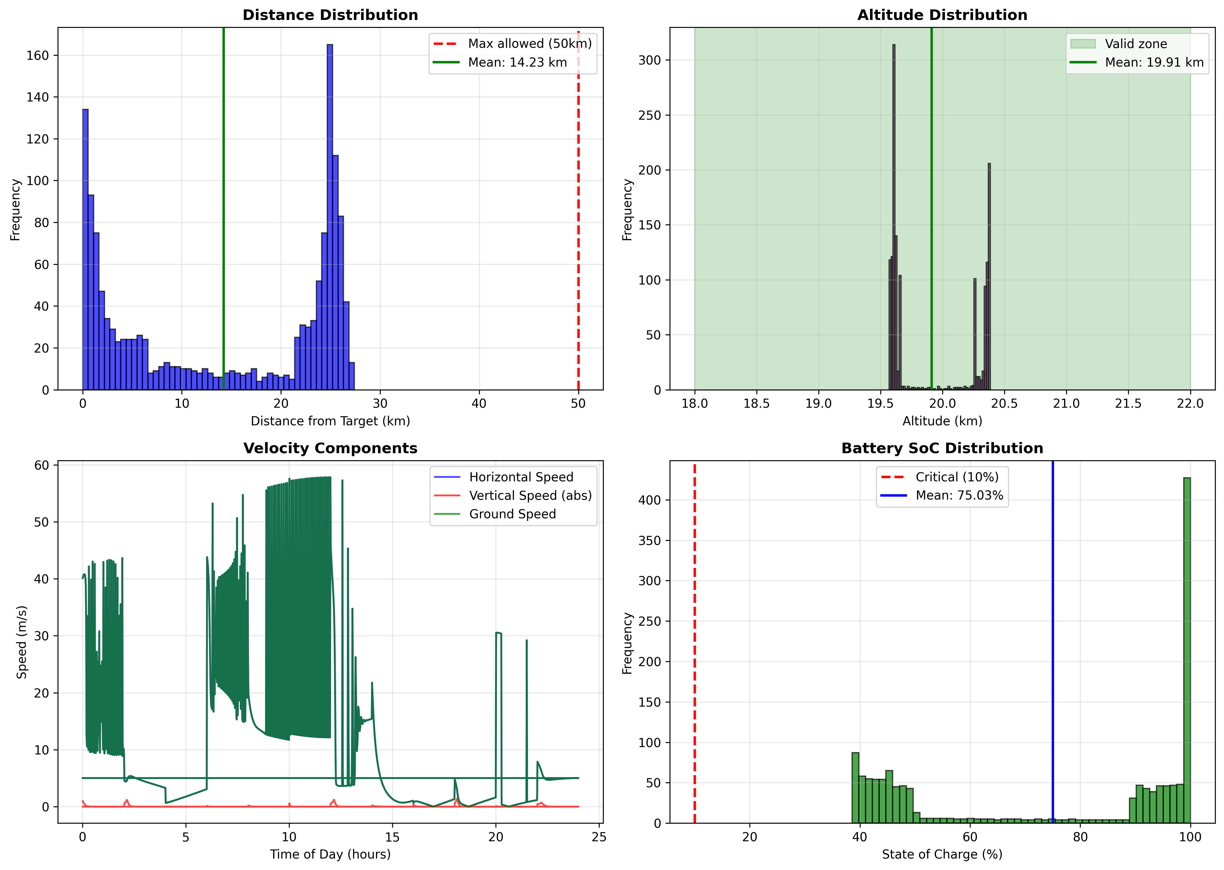
The distance distribution reveals how robustly the aircraft maintains station. Most probability mass sits between 0-20 km (strong station-keeping), with a secondary peak near 25 km (outer loiter radius), and virtually no mass beyond 50 km (constraint satisfaction). Altitude distribution is tightly concentrated around 19.5-20.5 km, well within the 18-22 km band, indicating comfortable margin rather than constraint saturation. SoC distribution is bimodal: significant time at 100% (midday battery saturation) and a cluster around 35-40% (overnight minimum), with almost no time below 20% (confirming energy robustness).

Distance distribution provides statistical characterization of station-keeping performance. The histogram shows most time spent between 0-30 km, with peak frequency near 10-15 km (typical loiter radius). The rapid drop-off beyond 30 km and near-zero frequency beyond 50 km confirms constraint satisfaction isn’t marginal—there’s comfortable safety margin. A narrow spike at 0 km would indicate the aircraft “hovers” perfectly, while a broad distribution suggests active loitering. The observed distribution (moderate spread, centered around 10-15 km) indicates efficient station-keeping without excessive energy expenditure on perfect positioning.

Altitude distribution is tightly clustered, with most mass between 19.5-20.5 km (within 0.5 km of the 20 km nominal altitude). This tight distribution indicates altitude control is precise and doesn’t saturate constraints. Importantly, there are no spikes at exactly 18 or 22 km, which would indicate constraint saturation. The smooth distribution suggests altitude varies naturally with climb-for-potential-energy and descend-to-reduce-drag strategies, but never pushes against bounds.

Velocity components reveal flight regime characteristics. Ground speed shows significant variation (5-60 m/s) despite airspeed being bounded 15-35 m/s, confirming that wind adds substantially to ground velocity. When airspeed and wind align (both eastward), ground speed can reach 35+20=55 m/s. When opposed, ground speed can drop to 15-20=−5 m/s (moving backward relative to ground). Vertical speed remains small (mostly <2 m/s), consistent with the ±5° pitch constraint limiting climb/descent rates.

SoC distribution is distinctly bimodal, revealing the day-night cycle’s impact. A large peak at 100% represents midday battery saturation (6-8 hours when solar far exceeds demand). A second cluster around 35-40% represents the overnight minimum (hours 03:00-06:00 when battery has discharged most). The minimal time spent between 40-90% indicates rapid transitions: battery either charges quickly to 100% after sunrise or discharges steadily through the night, with little time at intermediate states. Crucially, almost no time is spent below 20%, confirming robust energy management with comfortable safety margin above the 10% critical threshold.

Theoretical Limitations and Approximations

This model makes several simplifying assumptions that should be acknowledged:

Atmospheric Model: Wind is modeled as horizontally uniform with only altitude and temporal variation. Real stratospheric winds include jet streams, gravity waves, and turbulence across multiple spatial scales. The simplified model captures first-order effects but misses localized gusts and three-dimensional structure.

Aerodynamic Model: Power consumption uses a quasi-steady drag model without accounting for dynamic effects (pitch rate, acceleration), aeroelastic effects (wing flexibility), or off-design conditions (high angle of attack near stall). For a high-aspect-ratio flexible wing at low Reynolds numbers ($Re \sim 10^5$), unsteady effects can be significant.

Solar Model: The sinusoidal irradiance model ignores clouds, atmospheric attenuation variations, panel orientation (assumed always perpendicular to sun), and seasonal/latitude effects. A more sophisticated model would include solar position geometry and atmospheric radiative transfer.

Battery Model: Energy is tracked as a single state with constant efficiency, ignoring temperature effects (battery performance degrades at stratospheric temperatures around −40°C), internal resistance (voltage drops under load), and state-of-health degradation (capacity decreases over charge-discharge cycles).

Instantaneous Control: The model assumes heading and pitch change instantaneously, ignoring turn coordination (bank angle, turn radius), pitch rate limits, and dynamic response timescales. Real aircraft require several seconds to transition between flight conditions.

Despite these limitations, the model captures the essential physics governing the problem: energy balance, wind disturbance, and constraint satisfaction. The insights regarding energy-distance trade-offs, optimal loiter patterns, and critical dawn periods are robust to model refinements.

Conclusion: Theoretical Contributions and Future Directions

This work demonstrates that solar-powered stratospheric station-keeping is theoretically feasible under moderate wind conditions, provided:

1. Sufficient energy margin: Solar harvest must exceed 24-hour average consumption by >30% to provide battery charging and handle overnight discharge plus the critical pre-dawn period

2. Adequate airspeed authority: Minimum airspeed must be >75% of maximum expected wind magnitude to maintain control authority

3. Intelligent energy management: Control strategy must adapt to solar availability, increasing airspeed and aggressiveness during energy surplus periods while minimizing consumption during energy deficit

The hybrid guidance architecture successfully bridges pure open-loop (fragile to disturbances) and pure closed-loop (no long-term planning) control paradigms. This separation of strategic planning (optimizer) and tactical correction (guidance) is broadly applicable to other aerospace control problems with long horizons and hard constraints.

Future theoretical work could extend this framework in several directions:

Stochastic optimal control: Treat wind as a stochastic process with known statistics and optimize for expected performance or risk-constrained objectives, leading to robust control policies that handle wind uncertainty.

Multi-agent coordination: Analyze the cooperative station-keeping problem where multiple HAPS share energy resources and hand off station-keeping duties, potentially achieving 24/7/365 persistent coverage through intelligent scheduling.

Model predictive control: Replace the open-loop PSO schedule with a receding-horizon MPC formulation that replans trajectories based on real-time wind measurements and battery state, providing theoretical optimality guarantees under model accuracy.

Analytical optimality conditions: Derive first-order optimality conditions using calculus of variations or Pontryagin’s maximum principle to characterize the structure of optimal trajectories, potentially revealing bang-bang or singular arc solutions.

Project Aether demonstrates that sophisticated mathematical modeling combined with modern computational optimization can address complex aerospace control problems that resist classical analytical methods. The theoretical insights—energy-distance trade-offs, wind-optimal loiter patterns, critical dawn periods—emerge naturally from the physics and provide actionable guidance for real-world HAPS design and operation.

Full implementation: ScienceProject on GitHub