This problem unlike the previous posts, is more “recent” in some sense. However, I also encountered this problem in a MCM competition (Even though I have not enrolled). Like the problems in MCM, this problem is also quite interesting and challenging.

Problem Background

While some animal species exist outside of the usual male or female sexes, most species are substantially either male or female. Although many species exhibit a 1:1 sex ratio at birth, other species deviate from an even sex ratio. This is called adaptive sex ratio variation. For example, the temperature of the nest incubating eggs of the American alligator influences the sex ratios at birth.

The role of lampreys is complex. In some lake habitats, they are seen as parasites with a significant impact on the ecosystem, whereas lampreys are also a food source in some regions of the world, such as Scandinavia, the Baltics, and for some Indigenous peoples of the Pacific Northwest in North America.

The sex ratio of sea lampreys can vary based on external circumstances. Sea lampreys become male or female depending on how quickly they grow during the larval stage. These larval growth rates are influenced by the availability of food. In environments where food availability is low, growth rates will be lower, and the percentage of males can reach approximately 78% of the population. In environments where food is more readily available, the percentage of males has been observed to be approximately 56% of the population.

We focus on the question of sex ratios and their dependence on local conditions, specifically for sea lampreys. Sea lampreys live in lake or sea habitats and migrate up rivers to spawn. The task is to examine the advantages and disadvantages of the ability for a species to alter its sex ratio depending on resource availability. Your team should develop and examine a model to provide insights into the resulting interactions in an ecosystem.

Questions to examine include the following:

• What is the impact on the larger ecological system when the population of lampreys can alter its sex ratio?
• What are the advantages and disadvantages to the population of lampreys?
• What is the impact on the stability of the ecosystem given the changes in the sex ratios of lampreys?
• Can an ecosystem with variable sex ratios in the lamprey population offer advantages to others in the ecosystem, such as parasites?

Analysis

Well, to be honest, finishing this problem based on the background and answering the questions is not my cup of tea since I am not giving a answer paper to the MCM competition. However, studying the population dynamics of sea lampreys is quite interesting. The problem type is quite common and widely discussed in the field of ecology. For me, this problem is more about the prey-predator model. The prey-predator model is a type of mathematical model that describes the population dynamics of two species in an ecosystem. The model consists of two differential equations, one for the prey population and one for the predator population. The prey population is the species that is eaten by the predator, while the predator population is the species that eats the prey. The model describes how the populations of the two species change over time based on the interactions between them.

Mathematical Model

To say more about prey-predator model in this problem, one may review the prey-predator model or so-called Lotka-Volterra model. The Lotka-Volterra model is a mathematical model that describes the population dynamics of two species in an ecosystem. The model consists of two differential equations, one for the prey population and one for the predator population. The prey population is the species that is eaten by the predator, while the predator population is the species that eats the prey. The model describes how the populations of the two species change over time based on the interactions between them. Considering the following equations:

where:

• $x$ is the prey population
• $y$ is the predator population
• $\alpha$ is the growth rate of the prey population
• $\beta$ is the rate at which the predator population consumes the prey population
• $\delta$ is the rate at which the predator population grows by consuming the prey population
• $\gamma$ is the death rate of the predator population
• $t$ is time
• $\frac{dx}{dt}$ is the rate of change of the prey population over time
• $\frac{dy}{dt}$ is the rate of change of the predator population over time
• $xy$ is the interaction between the prey and predator populations

To solve the prey-predator model numerically, one may apply the Euler’s method or Runge-Kutta method. Both are discussed in the previous posts.

Solution

The solution of this problem, is quite complex and challenging. I consider this will ever be a research problem.

But any way, I will implement the prey-predator model in Python to simulate the population dynamics of sea lampreys.

# Importing the necessary libraries
import numpy as np
import matplotlib.pyplot as plt

import matplotlib as mpl
mpl.rcParams['axes.spines.right'] = False
mpl.rcParams['axes.spines.top'] = False
mpl.rcParams['axes.grid'] = True
mpl.rcParams['grid.color'] = '0.75'
mpl.rcParams['grid.linestyle'] = '--'
mpl.rcParams['grid.linewidth'] = 0.5
mpl.rcParams['font.size'] = 18
mpl.rcParams['axes.titlesize'] = 28

Since I want to include random noise in the model (One may think of the reason), I will use the numpy library to generate random numbers.

# Setting the random seed
np.random.seed(32)

Then I define a class called Organism to represent the population dynamics of the whole system in the ecosystem.

# Defining the Organism class
class Organism:
    def __init__(self, initial_population):
        self.population = initial_population

    def update_population(self, birth_rate, mortality_rate):
        self.population += int(self.population * (birth_rate - mortality_rate))
        self.population = max(0, self.population)

Next, I define another class called LampreyPopulation to represent the population dynamics of sea lampreys in the ecosystem.

# Defining the LampreyPopulation class
class LampreyPopulation(Organism):
    def __init__(self, initial_population, initial_food):
        super().__init__(initial_population)
        self.food = initial_food
        self.male_ratio = 0.5  # Initialize with a default value
        self.female_ratio = 0.5

    def update_sex_ratio(self, temperature):
        # Incorporate temperature effect on sex ratio
        temp_factor = max(0, min(1, (temperature - 10) / 20))  # Assume 10-30°C range
        self.male_ratio = max(0.56, min(0.78, 0.78 - 0.22 * (self.food / 1000) - 0.1 * temp_factor)*np.random.normal(1, 0.1))
        self.female_ratio = 1 - self.male_ratio

    def reproduce(self, birth_rate):
        return int(self.population * self.female_ratio * birth_rate)

    def update_population(self, predator_population, r, K, a):
        delta_lamprey = r * self.population * (1 - self.population / K) - a * predator_population * self.population / K
        self.population += int(delta_lamprey)
        self.population = max(0, self.population)

    def update_food(self, algae_population, food_consumption_rate):
        self.food = algae_population * 0.1  # Assume 10% of algae is edible for lampreys
        self.food -= self.population * food_consumption_rate
        self.food = max(0, self.food)

In the LampreyPopulation class, I have defined the following:

• update_sex_ratio: This function updates the sex ratio for sea lampreys based on the temperature
• reproduce: This function calculates the number of sea lampreys that reproduce based on the birth rate
• update_population: This function updates the population of sea lampreys based on the growth rate, carrying capacity, and predation rate
• update_food: This function updates the food availability for sea lampreys based on the algae population and food consumption rate

Following the LampreyPopulation class, I define another class called Predator to represent the population dynamics of predators in the ecosystem.

class Predator(Organism):
    def __init__(self, initial_population):
        super().__init__(initial_population)

    def update_population(self, lamprey_population, a, b, d, K):
        delta_predator = b * a * lamprey_population * self.population / K - d * self.population
        self.population += int(delta_predator)
        self.population = max(0, self.population)

    def hunt(self, lamprey_population, hunting_efficiency):
        return int(min(self.population * hunting_efficiency, lamprey_population * 0.1))

In the Predator class, one may see the implementation of prey-predator model in the update_population function.

Moreover, I define another class called Algae to represent the population dynamics of algae in the ecosystem.

# Defining the Algae class
class Algae(Organism):
    def __init__(self, initial_population, carrying_capacity):
        super().__init__(initial_population)
        self.carrying_capacity = carrying_capacity

    def grow(self, growth_rate, temperature, nutrient_level):
        temp_factor = max(0, min(1, (temperature - 5) / 25))
        nutrient_factor = min(1, nutrient_level / 100)
        effective_growth_rate = growth_rate * temp_factor * nutrient_factor
        self.population += int(self.population * effective_growth_rate * (1 - self.population / self.carrying_capacity))
        self.population = max(0, min(self.population, self.carrying_capacity))

Furthermore, I define a function called simulate_ecosystem to simulate the population dynamics of the ecosystem over time.

def simulate_ecosystem(years, lamprey, predator, algae, params):
    history = {
        'lamprey_pop': [], 'predator_pop': [], 'algae_pop': [],
        'male_ratio': [], 'temperature': [], 'nutrient_level': []
    }

    for year in range(years):
        temperature = 20 + 10 * np.sin(2 * np.random.uniform(0, 1) * np.pi * year / 4)
        
        params['nutrient_level'] += np.random.normal(0, 5)
        params['nutrient_level'] = max(0, min(100, params['nutrient_level']))

        algae.grow(params['algae_growth_rate'], temperature, params['nutrient_level'])
        lamprey.update_food(algae.population, params['food_consumption_rate'])
        lamprey.update_sex_ratio(temperature)

        lamprey.update_population(predator.population, params['lamprey_growth_rate'], params['lamprey_carrying_capacity'], params['predation_rate'])
        predator.update_population(lamprey.population, params['predation_rate'], params['predator_reproduction_rate'], params['predator_death_rate'], params['lamprey_carrying_capacity'])

        if year % 5 == 0:
            lamprey.population = int(lamprey.population * (1 - params['fishing_rate']))
            params['nutrient_level'] += params['pollution_rate'] * 10

        history['lamprey_pop'].append(lamprey.population)
        history['predator_pop'].append(predator.population)
        history['algae_pop'].append(algae.population)
        history['male_ratio'].append(lamprey.male_ratio)
        history['temperature'].append(temperature)
        history['nutrient_level'].append(params['nutrient_level'])

    return history

Equally important, we have established the whole model. Now, we can also set up the parameters for the simulation.

# Simulation parameters
params = {
    'lamprey_growth_rate': 0.3,
    'lamprey_carrying_capacity': 10000,
    'predation_rate': 0.2,
    'predator_reproduction_rate': 0.35,
    'predator_death_rate': 0.025,
    'algae_growth_rate': 0.1,
    'food_consumption_rate': 0.1,
    'nutrient_level': 50,
    'fishing_rate': 0.3,
    'pollution_rate': 0.2
}

# Initialize ecosystem
lamprey = LampreyPopulation(initial_population=1000, initial_food=2000)
predator = Predator(initial_population=100)
algae = Algae(initial_population=10000, carrying_capacity=50000)

We can then run the simulation for a specified number of years and visualize the results.

# Run simulation
years = 400
history = simulate_ecosystem(years, lamprey, predator, algae, params)

Finally, we can visualize the results of the simulation using matplotlib.

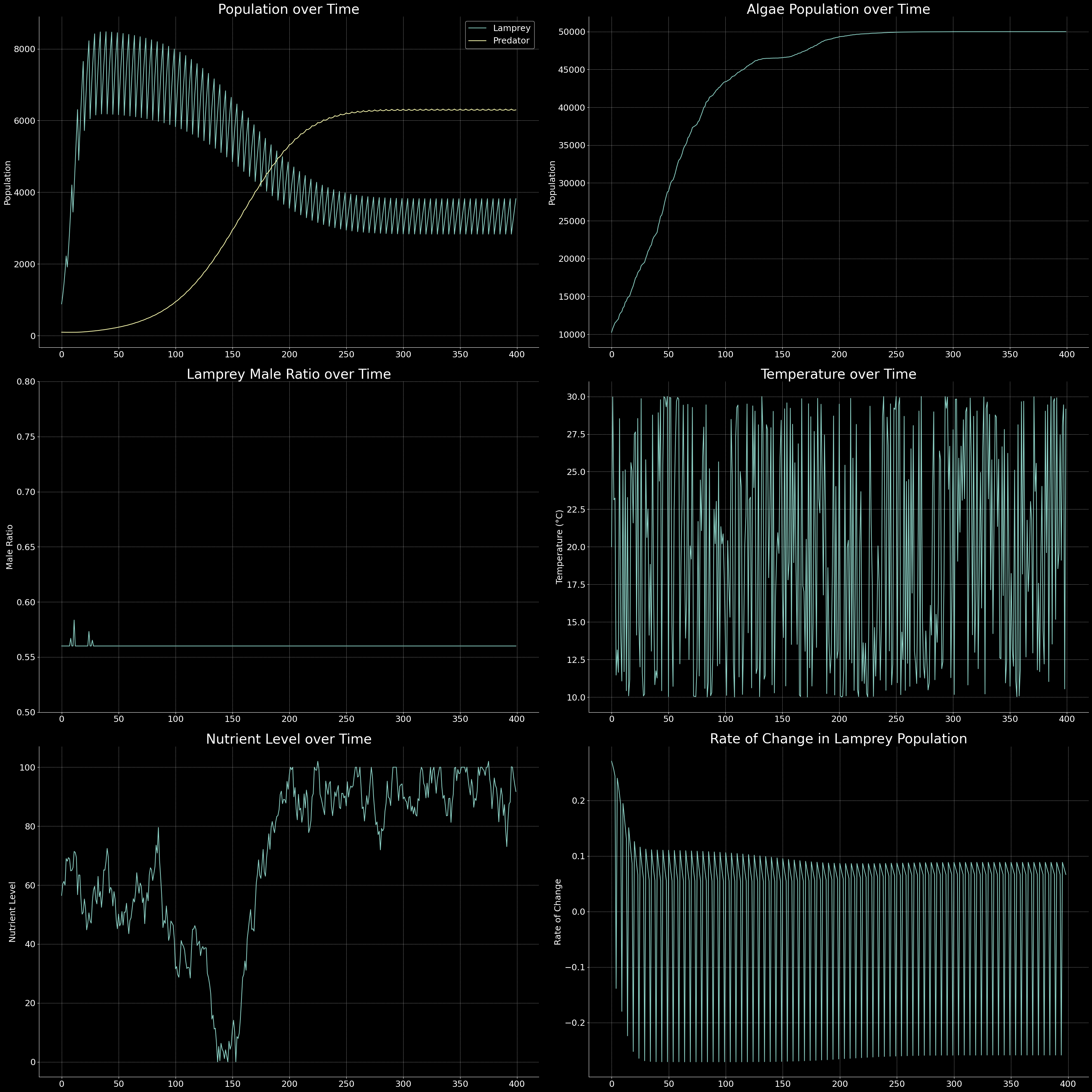
# Plotting results
fig, axes = plt.subplots(3, 2, figsize=(32, 32), dpi = 400)

axes[0, 0].plot(history['lamprey_pop'], label='Lamprey')
axes[0, 0].plot(history['predator_pop'], label='Predator')
axes[0, 0].set_title('Population over Time')
axes[0, 0].set_ylabel('Population')
axes[0, 0].legend()

axes[0, 1].plot(history['algae_pop'])
axes[0, 1].set_title('Algae Population over Time')
axes[0, 1].set_ylabel('Population')

axes[1, 0].plot(history['male_ratio'])
axes[1, 0].set_title('Lamprey Male Ratio over Time')
axes[1, 0].set_ylabel('Male Ratio')
axes[1, 0].set_ylim(0.5, 0.8)

axes[1, 1].plot(history['temperature'])
axes[1, 1].set_title('Temperature over Time')
axes[1, 1].set_ylabel('Temperature (°C)')

axes[2, 0].plot(history['nutrient_level'])
axes[2, 0].set_title('Nutrient Level over Time')
axes[2, 0].set_ylabel('Nutrient Level')

# Calculate and plot the rate of change in lamprey population
lamprey_pop_change = np.diff(history['lamprey_pop']) / np.array(history['lamprey_pop'][:-1])
axes[2, 1].plot(lamprey_pop_change)
axes[2, 1].set_title('Rate of Change in Lamprey Population')
axes[2, 1].set_ylabel('Rate of Change')

plt.tight_layout()
plt.show()

The code above will generate a plot showing the population dynamics of sea lampreys, predators, algae over time, are depicted in the following figure.

Conclusion

In a nutshell, this problem is about population dynamics of sea lampreys. The problem is quite interesting and challenging. The problem is more about the prey-predator model. The prey-predator model is a type of mathematical model that describes the population dynamics of two species in an ecosystem. The model consists of two differential equations, one for the prey population and one for the predator population. The model describes how the populations of the two species change over time based on the interactions between them.